A single attention head, built in Building Self-Attention Step by Step, computes one set of affinities per position: one way of deciding which earlier characters matter. This phase of the walkthrough turns it into a full Transformer block. It runs several heads in parallel, gives each position a small neural network of its own, wraps both in residual connections and layer normalization, and stacks the result. By the end of the phase the model has the complete architecture of the final GPT, still at toy size: 32-dimensional embeddings, 8 characters of context and 42,369 parameters.
The code for this phase is in steps/4_the_transformer_architecture. In this phase the step files are numbered exactly as the walkthrough's sections: file train_gpt_4_n.py implements section 4.n. Parameter counts come from tools/experiments/gpt/param_counts.py in this site's repository.
Multi-head attention
Reading Shakespeare, we track several things at once: grammar, who is speaking, the rhythm of the line. One attention head produces one weighting of the past per position, so it has to compromise between such concerns. Multi-head attention runs several heads side by side, each with its own query, key and value projections, so that each is free to learn a different pattern, and then concatenates their outputs and mixes them with a learned linear projection. Step file: train_gpt_4_1.py.
--- train_gpt_3_18.py
+++ train_gpt_4_1.py
@@ -123,2 +123,17 @@
 ####################################################################################################
+# Multi-Head Self-Attention
+
+class MultiHeadAttention(nn.Module):
+    def __init__(self, num_heads, head_size):
+        super().__init__()
+        self.heads = nn.ModuleList([SelfAttentionHead(head_size) for _ in range(num_heads)])
+        self.projection = nn.Linear(num_heads * head_size, C)  # Project back to C dimensions
+
+    def forward(self, x):
+        # Concatenate the outputs of all heads
+        out = torch.cat([head(x) for head in self.heads], dim=-1)
+        # Project back to original embedding size
+        return self.projection(out)
+
+####################################################################################################
 # The Bigram Language Model with Positional Embeddings
This is the multi-head attention of Vaswani et al. (2017, Section 3.2.2): $\text{MultiHead}(X) = \text{Concat}(\text{head}_1, \ldots, \text{head}_h)\, W^O$, where each head applies scaled dot-product attention to its own projections of the input. The authors' motivation is that multiple heads let the model "jointly attend to information from different representation subspaces at different positions", which a single head's averaging inhibits. They used 8 heads, each of dimension $d_{\text{model}}/h = 64$, so that the total cost is similar to one head of full width (Section 3.2.2). Their Table 3, rows (A), varies the number of heads at constant computation: one head was 0.9 BLEU worse than the best setting on their translation task, and quality also dropped with too many heads (Section 6.2).
The walkthrough's model follows the same rule of splitting the embedding among the heads. With $C = 32$ and four heads, each head has size $32 / 4 = 8$, the four outputs concatenate back to 32 dimensions, and the projection maps 32 to 32. Step file: train_gpt_4_2.py, whose model class now reads:
class BigramLanguageModel(nn.Module):
    def __init__(self):
        super().__init__()
        self.token_embedding_table = nn.Embedding(vocab_size, C)
        self.position_embedding_table = nn.Embedding(block_size, C)

        # Multi-head attention setup
        num_heads = 4
        head_size = C // num_heads
        self.multi_head_attention = MultiHeadAttention(num_heads, head_size)

        self.LM_head = nn.Linear(C, vocab_size)

    def forward(self, idx, targets=None):
        B, T = idx.shape

        # Token and positional embeddings
        token_embeddings = self.token_embedding_table(idx)
        position_idx = torch.arange(T, device=idx.device) % block_size
        positional_embeddings = self.position_embedding_table(position_idx)
        x = token_embeddings + positional_embeddings

        # Pass through multi-head attention
        x = self.multi_head_attention(x)

        # Pass through the language modeling head to get logits
        logits = self.LM_head(x)
        return logits
The four heads together have exactly as many query, key and value weights as the single 32-wide head they replace (4 × 3 × 32 × 8 = 3 × 32 × 32 = 3,072); the projection adds 32 × 32 + 32 = 1,056, for 8,609 parameters in all. One head might come to track the shapes of words, another the position within a line, another the capital letters of speaker names; which patterns the heads actually learn is not designed in, and is found only by inspecting a trained model.
The position-wise feedforward layer
Attention moves information between positions, but it is a weighted average: within a head, the output is a linear combination of value vectors. Each position also needs to process what it has gathered. The feedforward layer is a small two-layer network applied to every position separately and identically: a linear map that expands the $C$ features to $4C$, a ReLU nonlinearity, and a linear map back to $C$. Step file: train_gpt_4_3.py.
--- train_gpt_4_2.py
+++ train_gpt_4_3.py
@@ -138,2 +138,18 @@
 ####################################################################################################
+# Feedforward Layer
+
+class FeedForwardLayer(nn.Module):
+    def __init__(self):
+        super().__init__()
+        self.fc1 = nn.Linear(C, 4 * C)  # Expand to 4x the embedding size
+        self.fc2 = nn.Linear(4 * C, C)  # Project back down to embedding size
+        self.relu = nn.ReLU()  # ReLU non-linearity
+
+    def forward(self, x):
+        x = self.fc1(x)  # First linear transformation
+        x = self.relu(x)  # Apply ReLU
+        return self.fc2(x)  # Project back to original dimension
+
+
+####################################################################################################
 # The Bigram Language Model with Positional Embeddings
This is the position-wise feedforward network of the original Transformer, $\text{FFN}(x) = \max(0, x W_1 + b_1) W_2 + b_2$ (Vaswani et al., 2017, Equation 2), whose inner layer was four times wider than the model dimension (2,048 against 512, Section 3.3). The expansion gives each position room for a nonlinear computation, and ReLU, which zeroes negative values, is what makes it more than another linear map. At $C = 32$ the layer has 32 × 128 + 128 + 128 × 32 + 32 = 8,352 parameters, about twice as many as the attention it follows.
Adding the feedforward layer to the model
The model now applies attention and then the feedforward layer before the LM head. Step file: train_gpt_4_4.py, whose model class reads:
class BigramLanguageModel(nn.Module):
    def __init__(self):
        super().__init__()
        self.token_embedding_table = nn.Embedding(vocab_size, C)  # Embedding into C dimensions
        self.position_embedding_table = nn.Embedding(block_size, C)  # Positional Embeddings
        num_heads = 4  # Number of attention heads
        head_size = C // num_heads  # Size of each head (C is the total embedding dimension)
        self.multi_head_attention = MultiHeadAttention(num_heads, head_size)  # Multi-head attention
        self.feed_forward = FeedForwardLayer()  # Feedforward network
        self.LM_head = nn.Linear(C, vocab_size)  # Language Modeling Head

    def forward(self, idx, targets=None):
        B, T = idx.shape  # B: Batch size, T: Time steps

        # Token embeddings (B x T -> B x T x C)
        token_embeddings = self.token_embedding_table(idx)  # Shape (B, T, C)

        # Positional embeddings (T -> T x C)
        position_idx = torch.arange(T, device=idx.device) % block_size  # Use modulo to wrap around
        positional_embeddings = self.position_embedding_table(position_idx)  # Shape (T, C)

        # Combine token and positional embeddings
        x = token_embeddings + positional_embeddings  # Shape (B, T, C)

        # Pass through multi-head attention
        x = self.multi_head_attention(x)  # Shape (B, T, C)

        # Pass through feedforward layer
        x = self.feed_forward(x)  # Shape (B, T, C)

        # Pass the embeddings through the LM head to get logits
        logits = self.LM_head(x)  # Shape (B, T, vocab_size)

        return logits
The pipeline is: embed each character and its position, let positions exchange information through attention, let each position refine its own representation through the feedforward layer, and predict. The generate method is unchanged, including its crop to the last block_size characters. The model has 16,961 parameters.
The Transformer block: communication, then computation
Attention followed by a feedforward layer is the unit that Transformers repeat. Packaging the pair as a module, the Transformer block, makes the repetition easy. Karpathy's lecture describes the block as communication followed by computation: in attention, positions communicate; in the feedforward layer, each computes on its own. Step file: train_gpt_4_5.py.
--- train_gpt_4_4.py
+++ train_gpt_4_5.py
@@ -152,2 +152,18 @@

+####################################################################################################
+# Transformer Block
+
+class TransformerBlock(nn.Module):
+    def __init__(self, num_heads, head_size):
+        super().__init__()
+        self.multi_head_attention = MultiHeadAttention(num_heads, head_size)  # Multi-head attention
+        self.feed_forward = FeedForwardLayer()  # Feedforward network
+
+    def forward(self, x):
+        # Communication through multi-head attention
+        x = self.multi_head_attention(x)  # Shape (B, T, C)
+        # Computation through feedforward network
+        x = self.feed_forward(x)  # Shape (B, T, C)
+        return x
+
Stacking blocks
Stacking blocks lets later blocks work on what earlier ones produced. A plausible division of labour is that early blocks capture common letter combinations, middle ones the shapes of words, and later ones phrases or the conventions of verse and dialogue, much as a reader moves from letters to words to sentences, though nothing forces a trained model to divide the work this way. The model stacks three blocks with nn.Sequential, which feeds each block's output to the next. Step file: train_gpt_4_6.py.
--- train_gpt_4_5.py
+++ train_gpt_4_6.py
@@ -177,6 +177,13 @@
         self.position_embedding_table = nn.Embedding(block_size, C)  # Positional Embeddings
+
         num_heads = 4  # Number of attention heads
         head_size = C // num_heads  # Size of each head (C is the total embedding dimension)
-        self.multi_head_attention = MultiHeadAttention(num_heads, head_size)  # Multi-head attention
-        self.feed_forward = FeedForwardLayer()  # Feedforward network
+
+        # Stack multiple Transformer Blocks
+        self.transformer_blocks = nn.Sequential(
+            TransformerBlock(num_heads, head_size),  # First Transformer Block
+            TransformerBlock(num_heads, head_size),  # Second Transformer Block
+            TransformerBlock(num_heads, head_size)   # Third Transformer Block (you can add more)
+        )
+
         self.LM_head = nn.Linear(C, vocab_size)  # Language Modeling Head
@@ -196,7 +203,4 @@

-        # Pass through multi-head attention
-        x = self.multi_head_attention(x)  # Shape (B, T, C)
-
-        # Pass through feedforward layer
-        x = self.feed_forward(x)  # Shape (B, T, C)
+        # Pass through stacked Transformer Blocks
+        x = self.transformer_blocks(x)  # Shape (B, T, C)
Three blocks of 12,480 parameters each bring the model to 41,921. Depth has a cost beyond size: gradients must now flow back through three attention layers and three feedforward layers, each of which can shrink or distort them, and a deep plain stack is hard to train. The next three steps address this.
Residual connections
A residual connection adds a sub-layer's input to its output: instead of $x \leftarrow f(x)$, the block computes $x \leftarrow x + f(x)$. Each sub-layer then learns a change to make to its input rather than a complete replacement, and if a sub-layer is not yet useful, its input passes through intact. Step file: train_gpt_4_7.py.
--- train_gpt_4_6.py
+++ train_gpt_4_7.py
@@ -153,3 +153,3 @@
 ####################################################################################################
-# Transformer Block
+# Transformer Block with Residual Connections

@@ -162,7 +162,8 @@
     def forward(self, x):
-        # Communication through multi-head attention
-        x = self.multi_head_attention(x)  # Shape (B, T, C)
-        # Computation through feedforward network
-        x = self.feed_forward(x)  # Shape (B, T, C)
+        # Communication through multi-head attention with residual connection
+        x = x + self.multi_head_attention(x)  # Residual connection after self-attention
+        # Computation through feedforward network with residual connection
+        x = x + self.feed_forward(x)  # Residual connection after feedforward layer
         return x
+
The gradient benefit is direct. The derivative of $x + f(x)$ with respect to $x$ is the identity plus the derivative of $f$, so the gradient of the loss reaches every earlier layer through an uninterrupted path of additions, however small $f$'s own contribution. The residual path can be pictured as a stream running from the embeddings to the LM head, which each sub-layer reads from and adds to; each character's embedding flows through it, enriched by every block with contextual information. The original Transformer wraps each of its sub-layers this way (Vaswani et al., 2017, Section 3.1). Residual connections add no parameters.
An experiment with extra projection layers
The walkthrough's next step adds a linear $C \times C$ "projection" after the attention and after the feedforward layer in each block, with the stated purpose of bringing the outputs back to dimension $C$ so that the residual additions line up. Step file: train_gpt_4_8.py.
--- train_gpt_4_7.py
+++ train_gpt_4_8.py
@@ -153,3 +153,3 @@
 ####################################################################################################
-# Transformer Block with Residual Connections
+# Transformer Block with Projection Layers

@@ -160,10 +160,13 @@
         self.feed_forward = FeedForwardLayer()  # Feedforward network
+        self.attention_projection = nn.Linear(C, C)  # Projection after self-attention
+        self.feedforward_projection = nn.Linear(C, C)  # Projection after feedforward network

     def forward(self, x):
-        # Communication through multi-head attention with residual connection
-        x = x + self.multi_head_attention(x)  # Residual connection after self-attention
-        # Computation through feedforward network with residual connection
-        x = x + self.feed_forward(x)  # Residual connection after feedforward layer
+        # Communication through multi-head attention with residual connection and projection
+        x = x + self.attention_projection(self.multi_head_attention(x))  # Residual + Projection
+
+        # Computation through feedforward network with residual connection and projection
+        x = x + self.feedforward_projection(self.feed_forward(x))  # Residual + Projection
+
         return x
-
The dimensions already matched. MultiHeadAttention has had its own projection from num_heads * head_size to $C$ since step 4.1, and the feedforward layer's second linear map returns from $4C$ to $C$. In the lecture code these two layers are the projections back into the residual stream. The added layers are therefore a second linear map directly after a linear map, and the composition of two linear maps is a single linear map: they add 2 × 1,056 = 2,112 parameters per block (6,336 in all, 48,257 total) without letting the model compute anything new. The next step file removes them again, and the walkthrough's later code does not use them; the finished model is as if this step had not happened.
Layer normalization
As activations pass through many layers they can drift in scale, some features growing large while others shrink, which makes optimization harder. Layer normalization rescales each position's feature vector to a standard form. For a vector $x$ of $C$ features with mean $\mu$ and variance $\sigma^2$ (computed over those $C$ features), it outputs
$$\text{LN}(x)_i = \gamma_i \, \frac{x_i - \mu}{\sqrt{\sigma^2 + \epsilon}} + \beta_i,$$
where $\epsilon$ is a small constant for numerical safety and $\gamma, \beta$ are learned per-feature scale and shift ($2C$ parameters). Unlike batch normalization, which normalizes each feature using statistics across the examples in a batch, layer normalization uses only the position's own features, so it behaves the same for any batch size and identically during training and generation, when there is a batch of one. Step file: train_gpt_4_9.py, which also removes the extra projections of the previous step.
--- train_gpt_4_8.py
+++ train_gpt_4_9.py
@@ -160,12 +160,10 @@
         self.feed_forward = FeedForwardLayer()  # Feedforward network
-        self.attention_projection = nn.Linear(C, C)  # Projection after self-attention
-        self.feedforward_projection = nn.Linear(C, C)  # Projection after feedforward network
-
-    def forward(self, x):
-        # Communication through multi-head attention with residual connection and projection
-        x = x + self.attention_projection(self.multi_head_attention(x))  # Residual + Projection
-
-        # Computation through feedforward network with residual connection and projection
-        x = x + self.feedforward_projection(self.feed_forward(x))  # Residual + Projection
-
+        self.ln1 = nn.LayerNorm(C)  # LayerNorm before self-attention
+        self.ln2 = nn.LayerNorm(C)  # LayerNorm before feedforward network
+
+    def forward(self, x):
+        # Communication through multi-head attention with LayerNorm
+        x = x + self.multi_head_attention(self.ln1(x))  # Apply LayerNorm1 and residual connection
+        # Computation through feedforward network with LayerNorm
+        x = x + self.feed_forward(self.ln2(x))  # Apply LayerNorm2 and residual connection
         return x
The normalization is applied to the input of each sub-layer, inside the residual branch: $x \leftarrow x + \text{Attention}(\text{LN}_1(x))$ and $x \leftarrow x + \text{FFN}(\text{LN}_2(x))$. This "pre-norm" arrangement is not the original Transformer's: Vaswani et al. normalize after the addition, computing $\text{LayerNorm}(x + \text{Sublayer}(x))$ (2017, Section 3.1). GPT-2 moved layer normalization "to the input of each sub-block" (Radford et al., 2019, Section 2.3), and the lecture code, and this model, follow GPT-2. In the pre-norm form the residual stream itself is never normalized, so the uninterrupted additive path of the previous section is preserved.
The final layer normalization
GPT-2 also added "an additional layer normalization ... after the final self-attention block" (Radford et al., 2019, Section 2.3). In the pre-norm form the output of the last block would otherwise reach the LM head unnormalized. The last step of the phase adds it, just before the LM head. Step file: train_gpt_4_10.py.
--- train_gpt_4_9.py
+++ train_gpt_4_10.py
@@ -172,3 +172,3 @@
 ####################################################################################################
-# The Bigram Language Model with Positional Embeddings
+# The Bigram Language Model with Final LayerNorm

@@ -190,2 +190,3 @@

+        self.final_layer_norm = nn.LayerNorm(C)  # Final LayerNorm before the output
         self.LM_head = nn.Linear(C, vocab_size)  # Language Modeling Head
@@ -207,2 +208,5 @@
         x = self.transformer_blocks(x)  # Shape (B, T, C)
+
+        # Final LayerNorm before the output projection
+        x = self.final_layer_norm(x)  # Normalize before output

@@ -224,2 +228,3 @@
         return idx
+
The complete architecture
The model now has every component of the final GPT. The figure shows it with the final sizes, which the next phase sets; at this point $C = 32$, four heads of size 8, three blocks and a context of 8 characters.
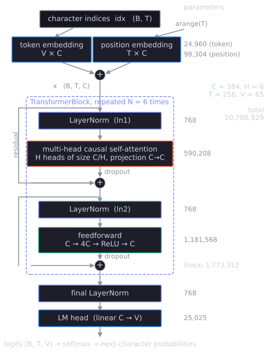
The parameter count through the phase:
| Step | Change | Parameters |
|---|---|---|
| 4.2 | four heads of size 8, with projection | 8,609 |
| 4.4 | feedforward layer | 16,961 |
| 4.6 | three blocks | 41,921 |
| 4.7 | residual connections | 41,921 |
| 4.8 | extra projections | 48,257 |
| 4.9 | layer normalization, extra projections removed | 42,305 |
| 4.10 | final layer normalization | 42,369 |
Compared with the Transformer of Vaswani et al. (2017), this is the decoder half alone, without the encoder and without the decoder's second attention layer, which attends to the encoder's output in translation; a model that only continues text has nothing to translate from. It uses learned rather than sinusoidal position vectors, pre-norm rather than post-norm layer normalization, and a final layer normalization, as GPT-2 does. The paper's base model has $d_{\text{model}} = 512$, 8 heads and 6 layers in each stack (Sections 3.1 and 3.2.2); the final model here has 384, 6 and 6. The next phase, Scaling the Shakespeare GPT, scales the model to those sizes and adds dropout.
References
- Karpathy, A. (2023). Let's build GPT: from scratch, in code, spelled out [Video lecture]. https://www.youtube.com/watch?v=kCc8FmEb1nY. Code: https://github.com/karpathy/ng-video-lecture
- Radford, A., Wu, J., Child, R., Luan, D., Amodei, D., and Sutskever, I. (2019). Language models are unsupervised multitask learners. OpenAI technical report. Cited: Section 2.3 (layer normalization at the input of each sub-block, final layer normalization).
- Vaswani, A., Shazeer, N., Parmar, N., Uszkoreit, J., Jones, L., Gomez, A. N., Kaiser, Ł., and Polosukhin, I. (2017). Attention is all you need. In Advances in Neural Information Processing Systems 30. arXiv:1706.03762. Cited: Section 3.1 (residual connections, post-norm), Section 3.2.2 (multi-head attention), Section 3.3 and Equation 2 (feedforward network), Section 6.2 and Table 3 (number of heads).
- Code for this article: gpt_text_model/steps/4_the_transformer_architecture in github.com/mdb42/ml-demos.