The The Bigram Language Model predicts each character from the one before it and ignores everything earlier. To do better, the representation of each position has to draw on the positions before it. This phase of the walkthrough builds the mechanism that does this, self-attention, in small steps: first the crudest form of token interaction, a plain average of the past; then the same average as one matrix product; then the average written so that its weights can be learned; and finally weights computed from the content of the tokens themselves. Along the way the model gets dense embeddings, a separate output layer and position information.
The code for this phase is in steps/3_the_attention_mechanism. Each code block is the difference between consecutive step files. The worked example's numbers come from tools/experiments/gpt/attention_example.py in this site's repository, and the figure from tools/figures/building-self-attention.py.
Averaging the past: a first form of token interaction
When we read "To be or not to", every earlier word shapes our expectation of the next. The simplest way to let a position draw on its history is to replace its vector with the average of the vectors at all positions up to and including it. For an input of shape (B, T, C) (batch, time, channels), the output at time $t$ is $\bar{x}_t = \frac{1}{t+1} \sum_{s=0}^{t} x_s$. This "bag of words" average discards order and treats every past character as equally important, but it is a mechanism through which tokens influence each other's representations, and every later step refines it. Step file: train_gpt_3_1.py.
--- train_gpt_2_9.py
+++ train_gpt_3_1.py
@@ -95,4 +95,25 @@
     def forward(self, idx, targets=None):
-        logits = self.token_embedding_table(idx)
+        # Embed the tokens (B x T -> B x T x C)
+        x = self.token_embedding_table(idx)  # Shape (B, T, C)
+
+        # Initialize the bag-of-words tensor (same shape as input data: B x T x C)
+        B, T, C = x.shape
+        X_bag_of_words = torch.zeros_like(x)
+
+        # Calculate feature vector by averaging the previous tokens
+        for b in range(B):
+            for t in range(T):
+                # Get all previous tokens (including the current token)
+                X_prev = x[b, :t + 1]  # (T_prev, C), where T_prev = t + 1
+
+                # Compute the average along the time dimension
+                feature_vector = X_prev.mean(dim=0)  # Shape (C)
+
+                # Store the result in X_bag_of_words
+                X_bag_of_words[b, t] = feature_vector
+
+        # (Optionally: proceed with other operations like generating logits)
+        logits = self.token_embedding_table(idx)  # Placeholder for next steps
         return logits
+
The averages are computed and then not used: the logits are still read from the token table, so the model's behaviour is unchanged. The first three steps of this phase are demonstrations of how to compute a causal average efficiently, written inside the forward pass so that the code is in place when the result is finally used. The double loop over batch and time is also slow: it performs B × T separate small operations in Python.
The same average as one matrix product
The average at every position can be computed at once with a matrix. Let $W$ be the $T \times T$ lower-triangular matrix of ones, so that row $t$ has ones in columns 0 to $t$ and zeros after. Dividing each row by its sum (the number of ones in it) gives row $t$ the weight $1/(t+1)$ on each of the first $t+1$ positions. Then the product $\bar{X} = W X$ computes every average simultaneously: row $t$ of $\bar{X}$ is $\sum_s W_{ts} x_s$, the average of $x_0, \ldots, x_t$. Step file: train_gpt_3_2.py.
--- train_gpt_3_1.py
+++ train_gpt_3_2.py
@@ -87,3 +87,3 @@
 ####################################################################################################
-# The Bigram Language Model
+# The Bigram Language Model with Vectorized Feature Calculation

@@ -98,22 +98,13 @@

-        # Initialize the bag-of-words tensor (same shape as input data: B x T x C)
+        # Vectorized computation using a lower triangular weight matrix for averaging
         B, T, C = x.shape
-        X_bag_of_words = torch.zeros_like(x)
+        W = torch.tril(torch.ones(T, T)).to(x.device)  # Lower triangular matrix of shape (T, T)
+        W = W / W.sum(dim=1, keepdim=True)  # Normalize to make sure each row sums to 1 for averaging

-        # Calculate feature vector by averaging the previous tokens
-        for b in range(B):
-            for t in range(T):
-                # Get all previous tokens (including the current token)
-                X_prev = x[b, :t + 1]  # (T_prev, C), where T_prev = t + 1
-
-                # Compute the average along the time dimension
-                feature_vector = X_prev.mean(dim=0)  # Shape (C)
-
-                # Store the result in X_bag_of_words
-                X_bag_of_words[b, t] = feature_vector
+        # Perform batched matrix multiplication: (B x T x T) @ (B x T x C) -> (B x T x C)
+        X_bag_of_words_2 = W @ x

         # (Optionally: proceed with other operations like generating logits)
-        logits = self.token_embedding_table(idx)  # Placeholder for next steps
+        logits = self.token_embedding_table(idx)  # Placeholder for further processing
         return logits
-
W has shape (T, T) and x has shape (B, T, C); PyTorch's batched matrix multiplication applies the same W to every sequence in the batch and returns shape (B, T, C). The hundreds of small Python operations become one matrix product, the kind of operation GPUs are built to execute.
The lower-triangular shape is the essential part. It encodes causality: position $t$ may draw on positions up to $t$ and never on later ones, because during generation later characters do not exist yet. The right-hand panel of the figure below shows this matrix for $T = 8$.
Softmax with a mask: averaging weights that can be learned
The matrix average weights every past position equally. Real text calls for unequal weights: some earlier characters matter more for the next one than others. The step that prepares for this writes the same averaging matrix a different way. Start from a matrix of zeros (in the code, the lower-triangular matrix of ones, whose values do not matter where they survive), set every entry above the diagonal to $-\infty$ with masked_fill, and apply softmax along each row. Step file: train_gpt_3_3.py.
--- train_gpt_3_2.py
+++ train_gpt_3_3.py
@@ -87,3 +87,3 @@
 ####################################################################################################
-# The Bigram Language Model with Vectorized Feature Calculation
+# The Bigram Language Model with Softmax-based Feature Calculation

@@ -98,12 +98,17 @@

-        # Vectorized computation using a lower triangular weight matrix for averaging
+        # Create a lower triangular matrix of ones
         B, T, C = x.shape
-        W = torch.tril(torch.ones(T, T)).to(x.device)  # Lower triangular matrix of shape (T, T)
-        W = W / W.sum(dim=1, keepdim=True)  # Normalize to make sure each row sums to 1 for averaging
+        Tril = torch.tril(torch.ones(T, T)).to(x.device)  # Lower triangular matrix of ones
+
+        # Mask future tokens by filling with -inf
+        W = Tril.masked_fill(Tril == 0, float('-inf'))  # Mask future tokens
+
+        # Apply softmax to compute normalized attention weights
+        W = F.softmax(W, dim=-1)

         # Perform batched matrix multiplication: (B x T x T) @ (B x T x C) -> (B x T x C)
-        X_bag_of_words_2 = W @ x
+        X_bag_of_words_3 = W @ x

-        # (Optionally: proceed with other operations like generating logits)
-        logits = self.token_embedding_table(idx)  # Placeholder for further processing
+        # Proceed with generating logits or further processing as needed
+        logits = self.token_embedding_table(idx)  # Placeholder for further steps
         return logits
Softmax turns a row of numbers $a_0, \ldots, a_{T-1}$ into positive weights $e^{a_s} / \sum_r e^{a_r}$ that sum to one. Since $e^{-\infty} = 0$, masked positions get weight exactly zero, which enforces causality: each position wears blinders and sees only what came before it. The unmasked entries in a row are all equal, so softmax gives them equal weights, $1/(t+1)$ each, and the result is the averaging matrix of the previous step.
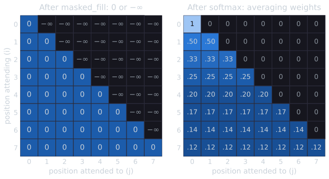
The point of the rewrite is the zeros. Here they are constants, so the weights are a fixed average. If they are replaced by numbers the model computes from the characters themselves, the same mask-and-softmax produces data-dependent weights that still respect causality and still sum to one. That replacement is self-attention, built below.
The walkthrough's text for this step also shows the constructor taking no arguments and using a new n_embed setting; in the step file those changes arrive in the next step, and this file still constructs the model with vocab_size.
Dense embeddings and a separate output layer
So far each character's vector has 65 entries, one per vocabulary item, read directly as next-character scores. The next step separates representation from prediction. Characters are embedded in a smaller, dense space of n_embed = 32 dimensions, whose values are learned; a linear layer then maps each 32-dimensional vector to 65 logits. Step file: train_gpt_3_6.py, which covers the walkthrough's sections on embedding dimensions and the linear layer.
--- train_gpt_3_3.py
+++ train_gpt_3_6.py
@@ -11,2 +11,3 @@
 block_size = 8
+n_embed = 32  # Number of embedding dimensions
 learning_rate = 1e-3
@@ -87,28 +88,17 @@
 ####################################################################################################
-# The Bigram Language Model with Softmax-based Feature Calculation
+# The Bigram Language Model

 class BigramLanguageModel(nn.Module):
-    def __init__(self, vocab_size):
+    def __init__(self):
         super().__init__()
-        self.token_embedding_table = nn.Embedding(vocab_size, vocab_size)
+        self.token_embedding_table = nn.Embedding(vocab_size, n_embed)  # Embedding into n_embed dimensions
+        self.linear_layer = nn.Linear(n_embed, vocab_size)  # Project embeddings back to vocab_size logits

     def forward(self, idx, targets=None):
-        # Embed the tokens (B x T -> B x T x C)
-        x = self.token_embedding_table(idx)  # Shape (B, T, C)
+        # Embed the tokens (B x T -> B x T x n_embed)
+        x = self.token_embedding_table(idx)  # Shape (B, T, n_embed)

-        # Create a lower triangular matrix of ones
-        B, T, C = x.shape
-        Tril = torch.tril(torch.ones(T, T)).to(x.device)  # Lower triangular matrix of ones
+        # Project embeddings to logits using the linear layer
+        logits = self.linear_layer(x)  # Shape (B, T, vocab_size)

-        # Mask future tokens by filling with -inf
-        W = Tril.masked_fill(Tril == 0, float('-inf'))  # Mask future tokens
-
-        # Apply softmax to compute normalized attention weights
-        W = F.softmax(W, dim=-1)
-
-        # Perform batched matrix multiplication: (B x T x T) @ (B x T x C) -> (B x T x C)
-        X_bag_of_words_3 = W @ x
-
-        # Proceed with generating logits or further processing as needed
-        logits = self.token_embedding_table(idx)  # Placeholder for further steps
         return logits
@@ -124,3 +114,3 @@

-model = BigramLanguageModel(vocab_size)
+model = BigramLanguageModel()
A one-hot vector, 64 zeros and a single one, says only which character this is. A learned 32-dimensional vector can place characters that behave alike near each other, for example vowels, or the capital letters that begin speaker names, in the same way that the The Vector Space Model places documents with similar terms near each other. The embedding compresses, and the linear layer expands back to scores over the vocabulary. With 32 dimensions the model has 65 × 32 = 2,080 embedding weights and 32 × 65 + 65 = 2,145 weights and biases in the linear layer, 4,225 in total, by coincidence exactly as many as the 65 × 65 table it replaces. The step also removes the averaging demonstrations, which return in their final form below.
The language-modeling head
The next step renames two things to match common usage. The embedding size n_embed becomes C (for "channels"), and the output layer becomes LM_head, the language-modeling head: the final linear layer of a language model, which turns the processed representation at each position into logits over the vocabulary. Step file: train_gpt_3_7.py.
--- train_gpt_3_6.py
+++ train_gpt_3_7.py
@@ -11,3 +11,3 @@
 block_size = 8
-n_embed = 32  # Number of embedding dimensions
+C = 32  # Embedding dimensions (renamed from n_embed to C)
 learning_rate = 1e-3
@@ -93,11 +93,11 @@
         super().__init__()
-        self.token_embedding_table = nn.Embedding(vocab_size, n_embed)  # Embedding into n_embed dimensions
-        self.linear_layer = nn.Linear(n_embed, vocab_size)  # Project embeddings back to vocab_size logits
+        self.token_embedding_table = nn.Embedding(vocab_size, C)  # Embedding into C dimensions (renamed from n_embed)
+        self.LM_head = nn.Linear(C, vocab_size)  # Language Modeling Head (embedding -> vocab_size)

     def forward(self, idx, targets=None):
-        # Embed the tokens (B x T -> B x T x n_embed)
-        x = self.token_embedding_table(idx)  # Shape (B, T, n_embed)
+        # Embed the tokens (B x T -> B x T x C)
+        x = self.token_embedding_table(idx)  # Shape (B, T, C)

-        # Project embeddings to logits using the linear layer
-        logits = self.linear_layer(x)  # Shape (B, T, vocab_size)
+        # Pass the embeddings through the LM head to get logits
+        logits = self.LM_head(x)  # Shape (B, T, vocab_size)
The model now has the shape every later version keeps: an embedding layer, some processing (none yet), and the LM head. Everything added from here on goes between the two.
Positional embeddings
Order matters in language: "To be or not to be" and "be to or be not to" use the same characters. An average or a weighted sum over positions, however, is the same whatever order its terms are in, so a model built only from them cannot tell where a character is. Positional embeddings fix this by giving each position $0, 1, \ldots, T-1$ its own learned vector, which is added to the character's embedding. The sum carries both what the character is and where it stands. Step file: train_gpt_3_8.py.
--- train_gpt_3_7.py
+++ train_gpt_3_8.py
@@ -11,3 +11,3 @@
 block_size = 8
-C = 32  # Embedding dimensions (renamed from n_embed to C)
+C = 32  # Embedding dimensions
 learning_rate = 1e-3
@@ -88,3 +88,3 @@
 ####################################################################################################
-# The Bigram Language Model
+# The Bigram Language Model with Positional Embeddings

@@ -93,8 +93,18 @@
         super().__init__()
-        self.token_embedding_table = nn.Embedding(vocab_size, C)  # Embedding into C dimensions (renamed from n_embed)
-        self.LM_head = nn.Linear(C, vocab_size)  # Language Modeling Head (embedding -> vocab_size)
+        self.token_embedding_table = nn.Embedding(vocab_size, C)  # Embedding into C dimensions
+        self.position_embedding_table = nn.Embedding(block_size, C)  # Positional Embeddings
+        self.LM_head = nn.Linear(C, vocab_size)  # Language Modeling Head

     def forward(self, idx, targets=None):
-        # Embed the tokens (B x T -> B x T x C)
-        x = self.token_embedding_table(idx)  # Shape (B, T, C)
+        B, T = idx.shape  # B: Batch size, T: Time steps
+
+        # Token embeddings (B x T -> B x T x C)
+        token_embeddings = self.token_embedding_table(idx)  # Shape (B, T, C)
+
+        # Positional embeddings (T -> T x C)
+        position_idx = torch.arange(T, device=idx.device) % block_size  # Use modulo to wrap around
+        positional_embeddings = self.position_embedding_table(position_idx)  # Shape (T, C)
+
+        # Combine token and positional embeddings
+        x = token_embeddings + positional_embeddings  # Shape (B, T, C)
The token embeddings have shape (B, T, C) and the positional embeddings (T, C); broadcasting adds the same position vectors to every sequence in the batch. Vaswani et al. (2017, Section 3.5) used fixed sinusoidal encodings in the original Transformer, and reported that learned positional embeddings, the kind used here, "produced nearly identical results" (Section 3.5; Table 3, row E). They chose sinusoids because these might extrapolate to sequences longer than those seen in training; learned embeddings cannot, since there is no vector for a position beyond block_size.
That limit explains the % block_size in the code. The position table has only block_size = 8 rows, but generation grows the sequence to 101 characters (one starting character and 100 new ones), and position 8 would be out of range. The modulo wraps positions around (8 becomes 0, 9 becomes 1) so the lookup never fails. The walkthrough's text presents the proper fix in this same section: crop the context to the last block_size characters before each prediction. In the step files that crop arrives later, in step 3_17, where it becomes necessary (see below).
Queries, keys and values
Self-attention computes, for each position, how much to draw on each earlier position from the content of the characters. Each position's vector $x$ is projected three ways by learned linear maps:
- a query $q = x W^Q$, what this position is looking for;
- a key $k = x W^K$, what this position offers to others;
- a value $v = x W^V$, the information it passes on if attended to.
The affinity between position $i$ and an earlier position $j$ is the dot product $q_i \cdot k_j$: large when the query and key point the same way. This is the same measure of agreement between vectors that underlies the Cosine Similarity of the vector space model, without the normalization by length. Collecting the queries and keys of all positions into matrices $Q$ and $K$ (one row per position), all affinities at once are $Q K^\top$, a $T \times T$ matrix, which takes the place of the zeros in the previous section's mask-and-softmax.
The walkthrough builds the head in pieces (projections; affinities; mask and softmax; weighted sum of values) across sections 3.8 to 3.12. The step file contains the finished head. Step file: train_gpt_3_13.py.
--- train_gpt_3_8.py
+++ train_gpt_3_13.py
@@ -88,2 +88,34 @@
 ####################################################################################################
+# The Self-Attention Head
+class SelfAttentionHead(nn.Module):
+    def __init__(self, head_size):
+        super().__init__()
+        self.head_size = head_size
+        self.query = nn.Linear(C, head_size, bias=False)  # Linear transformation for queries
+        self.key = nn.Linear(C, head_size, bias=False)    # Linear transformation for keys
+        self.value = nn.Linear(C, head_size, bias=False)  # Linear transformation for values
+
+    def forward(self, x):
+        B, T, C = x.shape
+
+        # Compute queries, keys, and values
+        Q = self.query(x)  # Shape (B, T, head_size)
+        K = self.key(x)    # Shape (B, T, head_size)
+        V = self.value(x)  # Shape (B, T, head_size)
+
+        # Compute affinities (Q dot K^T)
+        affinities = Q @ K.transpose(-2, -1) / (self.head_size ** 0.5)  # Shape (B, T, T)
+
+        # Dynamically create a mask for future tokens
+        mask = torch.tril(torch.ones(T, T, device=x.device))  # Shape (T, T)
+        affinities = affinities.masked_fill(mask == 0, float('-inf'))
+
+        # Apply softmax to get attention weights
+        attention_weights = F.softmax(affinities, dim=-1)  # Shape (B, T, T)
+
+        # Aggregate values based on attention weights
+        out = attention_weights @ V  # Shape (B, T, head_size)
+        return out
+
+####################################################################################################
 # The Bigram Language Model with Positional Embeddings
In one formula, with $M$ the mask (0 on and below the diagonal, $-\infty$ above) and $d_k$ the head size, the head computes
$$\text{head}(X) = \operatorname{softmax}\!\left(\frac{Q K^\top}{\sqrt{d_k}} + M\right) V, \qquad Q = X W^Q,\; K = X W^K,\; V = X W^V,$$
which is the scaled dot-product attention of Vaswani et al. (2017, Equation 1), with the decoder's masking: "masking out (setting to −∞) all values in the input of the softmax which correspond to illegal connections" (Section 3.2.3). The projections have no bias (bias=False), as in the lecture code. The query-key-value split is like a library search: the query is the question, the keys are the catalogue entries it is matched against, and the values are the contents of the books, mixed into the answer in proportion to how well each entry matched.
A worked example of masked attention
Take three positions and a head size of 2, with hand-picked queries, keys and values (learned ones would be arbitrary-looking numbers; these keep the arithmetic visible):
| Position | $q$ | $k$ | $v$ |
|---|---|---|---|
| 0 | (1, 0) | (2, 0) | (1, 0) |
| 1 | (0, 2) | (0, 1) | (0, 1) |
| 2 | (1, 1) | (1, 1) | (1, 1) |
Affinities. $Q K^\top$ has entry $(i, j) = q_i \cdot k_j$. Row 0 is $(2, 0, 1)$, row 1 is $(0, 2, 2)$ and row 2 is $(2, 1, 2)$.
Scaling. Dividing by $\sqrt{2} \approx 1.4142$ gives rows $(1.4142, 0, 0.7071)$, $(0, 1.4142, 1.4142)$ and $(1.4142, 0.7071, 1.4142)$.
Mask. Entries above the diagonal become $-\infty$: position 0 keeps only its own score 1.4142; position 1 keeps $(0, 1.4142)$; position 2 keeps all three. Note that position 0's affinity with position 2 (0.7071) and position 1's with position 2 (1.4142) are discarded: they would let the past see the future.
Softmax. Row 0 becomes $(1, 0, 0)$. Row 1: $e^0 = 1$ and $e^{1.4142} = 4.113$, so the weights are $1/5.113 = 0.1956$ and $4.113/5.113 = 0.8044$. Row 2: $e^{1.4142} = 4.113$ twice and $e^{0.7071} = 2.028$, total 10.254, so the weights are $(0.4011, 0.1978, 0.4011)$. Each row sums to 1.
Weighted sum of values. Position 0 outputs $v_0 = (1, 0)$. Position 1 outputs $0.1956\,(1, 0) + 0.8044\,(0, 1) = (0.1956, 0.8044)$, drawing mostly on itself because its query $(0, 2)$ matches its own key $(0, 1)$ better than position 0's key $(2, 0)$. Position 2 outputs $0.4011\,(1,0) + 0.1978\,(0,1) + 0.4011\,(1,1) = (0.8022, 0.5989)$.
All values are rounded to four decimals. The output at each position is a mixture of the values of the positions it may see, in proportions decided by query-key agreement.
Self-attention in principle lets a position reach back to any earlier position, but in this model it can reach only as far as the context allows. With block_size = 8, the model sees at most eight characters, so it could not, for instance, connect "me" in "Friends, Romans, countrymen, lend me your ears" back to the opening words, or recall the earlier "to be" when completing "to be or not to b". Those are the kinds of dependencies that attention makes possible once the context is long enough, as in Scaling the Shakespeare GPT, where it is 256 characters.
Putting the attention head into the model
The next step inserts one attention head between the embeddings and the LM head, with a head size equal to the embedding size, 32, so that its output can go straight to the LM head. Step file: train_gpt_3_14.py.
--- train_gpt_3_13.py
+++ train_gpt_3_14.py
@@ -127,2 +127,3 @@
         self.position_embedding_table = nn.Embedding(block_size, C)  # Positional Embeddings
+        self.attention_head = SelfAttentionHead(C)  # Self-attention head with the same size as embeddings
         self.LM_head = nn.Linear(C, vocab_size)  # Language Modeling Head
@@ -141,2 +142,5 @@
         x = token_embeddings + positional_embeddings  # Shape (B, T, C)
+
+        # Pass through self-attention head
+        x = self.attention_head(x)  # Shape (B, T, C)
Information now flows as follows: each character gets a token embedding plus a positional embedding; the attention head lets each position gather information from the positions before it; and the LM head turns each position's result into next-character scores. Where the bigram model saw one character back, each position now sees up to eight. The model has 7,553 parameters: 2,080 for the token embeddings, 256 (8 × 32) for the positions, 3,072 (three 32 × 32 projections) for the head, and 2,145 for the LM head.
Why the dot products are scaled
The division by $\sqrt{d_k}$ was already in the head's code; the walkthrough explains it in its own section, and the corresponding step file (train_gpt_3_15.py) changes only the comments.
The reason is the size of dot products. If the components of $q$ and $k$ are independent with mean 0 and variance 1, their dot product $q \cdot k = \sum_{i=1}^{d_k} q_i k_i$ is a sum of $d_k$ terms of variance 1, so it has mean 0 and variance $d_k$ (Vaswani et al., 2017, Section 3.2.1 and footnote 4). Its typical size grows like $\sqrt{d_k}$. Vaswani et al. suspected that such large scores push softmax into regions where it puts almost all the weight on one position and its gradients are extremely small, which slows learning. Dividing by $\sqrt{d_k}$ brings the variance back to 1 for every head size.
A simulation with 8 positions shows the effect, drawing each unscaled score independently from a normal distribution with mean 0 and variance $d_k$ (one seeded run of 20,000 rows, in attention_example.py). Unscaled, the median of the largest softmax weight is 0.664 for $d_k = 8$, 0.965 for $d_k = 64$ and 1.000 for $d_k = 512$: the bigger the head, the closer attention comes to a hard choice. Scaled, it is about 0.33 for all three. Scaling never sharpens attention; for any head size above 1 it only divides the scores down, so it guards against overly peaked weights, not overly flat ones.
Registering the mask as a buffer
The mask depends only on the sequence length, so there is no need to rebuild it on every forward pass. The next step creates it once, at full block_size, and registers it with register_buffer, which makes it part of the module's state (it moves to the GPU with the model and is saved with it) without making it a trainable parameter. The forward pass slices the top-left $T \times T$ corner for shorter inputs. Step file: train_gpt_3_16.py.
--- train_gpt_3_15.py
+++ train_gpt_3_16.py
@@ -93,5 +93,9 @@
         self.head_size = head_size
-        self.query = nn.Linear(C, head_size, bias=False)  # Linear transformation for queries
-        self.key = nn.Linear(C, head_size, bias=False)    # Linear transformation for keys
-        self.value = nn.Linear(C, head_size, bias=False)  # Linear transformation for values
+        self.query = nn.Linear(C, head_size, bias=False)
+        self.key = nn.Linear(C, head_size, bias=False)
+        self.value = nn.Linear(C, head_size, bias=False)
+
+        # Register triangular mask as a buffer
+        mask = torch.tril(torch.ones(block_size, block_size))
+        self.register_buffer('mask', mask)

@@ -106,7 +110,6 @@
         # Compute affinities (Q dot K^T) and apply scaling
-        affinities = Q @ K.transpose(-2, -1) / (self.head_size ** 0.5)  # Scale by sqrt(head_size)
+        affinities = Q @ K.transpose(-2, -1) / (self.head_size ** 0.5)

         # Apply triangular mask to prevent future tokens from communicating
-        mask = torch.tril(torch.ones(T, T, device=x.device))  # Shape (T, T)
-        affinities = affinities.masked_fill(mask == 0, float('-inf'))
+        affinities = affinities.masked_fill(self.mask[:T, :T] == 0, float('-inf'))
Cropping the context during generation
The buffered mask has a side effect the walkthrough's text does not mention. Generation grows the sequence to 101 characters, but the buffer has only 8 rows and columns, so for inputs longer than 8 the slice self.mask[:T, :T] is still 8 × 8 and no longer matches the $T \times T$ affinities; the previous step file's generation code therefore fails. The fix is the crop the walkthrough describes with positional embeddings: before each prediction, keep only the last block_size characters. Step file: train_gpt_3_17.py.
--- train_gpt_3_16.py
+++ train_gpt_3_17.py
@@ -156,3 +156,6 @@
         for _ in range(max_new_tokens):
-            logits = self(idx)
+            # Crop context if it exceeds block size
+            idx_cond = idx if idx.size(1) <= block_size else idx[:, -block_size:]
+
+            logits = self(idx_cond)
             logits = logits[:, -1, :]
@@ -162,2 +165,3 @@
         return idx
+
The crop also makes the % block_size wrap-around in the positional embeddings unnecessary, since positions never exceed block_size - 1 again; the modulo stays in the code to the end, harmless.
A lower learning rate
The walkthrough closes this phase by suggesting experiments with the learning rate. The last step file of the phase lowers it from 1e-3 to 1e-4. Step file: train_gpt_3_18.py.
--- train_gpt_3_17.py
+++ train_gpt_3_18.py
@@ -12,3 +12,3 @@
 C = 32  # Embedding dimensions
-learning_rate = 1e-3
+learning_rate = 1e-4
 eval_interval = 100
This completes a single head of masked self-attention. One head computes one pattern of affinities per position, a single way of deciding what matters. The next phase, Assembling the Transformer Block, runs several heads in parallel and adds the rest of the Transformer block around them.
References
- Karpathy, A. (2023). Let's build GPT: from scratch, in code, spelled out [Video lecture]. https://www.youtube.com/watch?v=kCc8FmEb1nY. Code: https://github.com/karpathy/ng-video-lecture
- Vaswani, A., Shazeer, N., Parmar, N., Uszkoreit, J., Jones, L., Gomez, A. N., Kaiser, Ł., and Polosukhin, I. (2017). Attention is all you need. In Advances in Neural Information Processing Systems 30. arXiv:1706.03762. Cited: Section 3.2.1 and Equation 1 (scaled dot-product attention), footnote 4 (variance of $q \cdot k$), Section 3.2.3 (masking), Section 3.5 and Table 3 row E (positional encodings).
- Code for this article: gpt_text_model/steps/3_the_attention_mechanism in github.com/mdb42/ml-demos.