A test collection measures a system against fixed judgments made by assessors. A search engine with millions of users can measure something closer to what it actually cares about: how real people respond to its results. If a new ranking function leads users to find what they want sooner and come back more often, it is better for those users, whatever the assessors would have said. Online evaluation compares systems by exposing them to live traffic and measuring behavior. It is how large search services and online stores decide whether to ship a change.
A/B testing
The simplest design is the controlled experiment, or A/B test. Users are randomly assigned to two groups. The control group sees the current system, the treatment group sees the new one, and the groups' behavior is compared over days or weeks. Random assignment ensures that any difference in behavior beyond chance is caused by the change, the same logic as a clinical trial (Kohavi, Longbotham, Sommerfield, and Henne, 2009).
Typical metrics for search include:
- Click rate: the fraction of queries with at least one click on a result. (Click-through rate more often means clicks per result shown, and definitions vary.)
- Time to first click, and rank of first click: how quickly users find something worth opening.
- Reformulation rate: how often users immediately rewrite a query, a sign the first results failed.
- Satisfied clicks: clicks after which the user stays on the page for a while, often defined by a dwell time threshold such as 30 seconds, rather than returning at once. Fox and colleagues (2005) found dwell time and how a session ended to be among the best behavioral predictors of users' own satisfaction ratings.
- Session and long-term metrics: queries per session, sessions per user, and whether users come back.
A/B tests need large samples. Behavioral metrics are noisy, users differ greatly from one another, and the effect of a single ranking change is usually small, so detecting it reliably can take millions of queries.
How many users?
How large an experiment must be follows from the same reasoning as the topic-count calculation in significance testing, with users in place of topics. Suppose the metric is a click rate. Each user in a group of $n$ either clicks (1) or does not (0), with probability $p$; one user's outcome has variance $\sigma^2 = p(1 - p)$, and the group's observed rate has variance $\sigma^2/n$. The difference between the two groups' rates, the quantity tested, has variance $2\sigma^2/n$ when the groups are the same size.
- The test. Declare a difference when the observed difference is more than $z_{1-\alpha/2}$ standard errors from zero: 1.96 for a two-sided test at $\alpha = 0.05$.
- The power. If the true difference is $\Delta$, the observed difference is centred on $\Delta$. It clears the threshold with probability $1 - \beta$ when $\Delta$ sits $z_{1-\beta}$ standard errors beyond it, that is, when $\Delta = (z_{1-\alpha/2} + z_{1-\beta}) \sqrt{2\sigma^2/n}$. For 80% power, $z_{0.8} = 0.842$.
- Solve for $n$:
$$n = \frac{2 (z_{1-\alpha/2} + z_{1-\beta})^2 \sigma^2}{\Delta^2} = \frac{2 (1.960 + 0.842)^2 \sigma^2}{\Delta^2} = \frac{15.7\, \sigma^2}{\Delta^2} \approx \frac{16\, \sigma^2}{\Delta^2}.$$
The last form is the rule of thumb Kohavi, Longbotham, Sommerfield, and Henne (2009, §3.2, equation 2) give for 95% confidence and 80% power, with $n$ the number of users in each group.
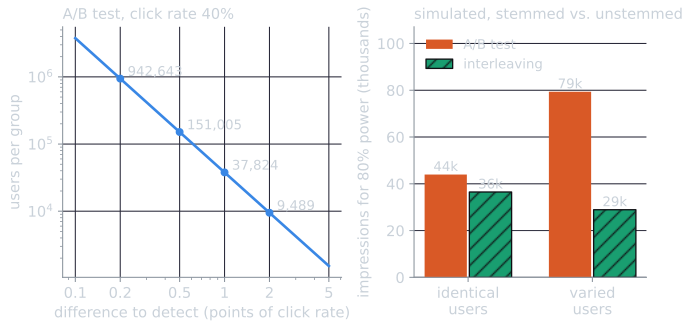
For a click rate of 40 percent, $\sigma^2 = 0.4 \times 0.6 = 0.24$. Detecting an improvement of one percentage point, to 41 percent, needs $16 \times 0.24/0.01^2 = 38{,}400$ users per group by the rule, or 37,824 by the exact formula using both groups' variances. The script tools/experiments/online/online_examples.py computes the table and checks it by simulation:
| Improvement to detect | Relative change | Users per group (exact) | Rule of thumb |
|---|---|---|---|
| 2 points (40% to 42%) | 5% | 9,489 | 9,600 |
| 1 point | 2.5% | 37,824 | 38,400 |
| 0.5 points | 1.25% | 151,005 | 153,600 |
| 0.2 points | 0.5% | 942,643 | 960,000 |
The required sample grows with the inverse square of the difference: halving the difference to detect quadruples the users, and detecting a 0.2-point change takes nearly a million users in each group. This is why a large service can detect a change too small for a smaller one to see, and why Kohavi and colleagues stress choosing metrics with low variance (§3.2). In simulation, 30 runs of 2,000 experiments with 38,400 users per group and a true difference of one point detected it in 80.5 percent of experiments (median; IQR 80.0 to 81.1), and with no true difference declared one in 5.0 percent, as designed.
The formula treats each user as one independent observation. When the unit randomized is the user but the metric is computed per query, a user's queries are correlated, and the variance must be computed per user, not per query, or the test will be overconfident.
What behavior means
Behavior is evidence about relevance, but indirect and biased evidence:
- Position bias. Users click higher results more often regardless of their quality, as described in relevance. A raw click count largely measures where results were placed.
- Snippet attraction. A click shows that the snippet looked promising, not that the page was good. A misleading snippet attracts clicks and disappoints.
- Good abandonment. A query with no clicks may mean failure, or it may mean the answer was on the results page itself, in a snippet or an answer box. Li, Huffman, and Tokuda (2009) found such good abandonment to be common, especially on mobile devices. A metric that counts every no-click query as a failure penalizes systems for answering questions directly.
- Metric gaming. A change can raise a metric without helping users, for example by making snippets more enticing but less accurate. Metrics need guardrails, secondary metrics that would reveal such side effects.
Because of these effects, online metrics are chosen and validated carefully, often by checking that they agree with explicit user satisfaction ratings in smaller studies.
Position bias, measured and modelled
Joachims, Granka, Pan, Hembrooke, and Gay (2005) separated position from quality with an eye tracker and a deliberate manipulation. Students searched with Google while their gaze was recorded. The abstracts at ranks 1 and 2 were viewed almost equally often, yet the first was clicked substantially more (§4.1). In one condition the top two results were swapped before display. Users still favoured whatever appeared first: in the swapped condition, among searches where the second abstract had been judged more relevant and the user clicked exactly one of the top two, 10 of 17 clicks went to the first, less relevant, abstract (§5.2.1, Table 3). The authors called this trust bias: users rely on the engine's ordering as well as on what they read.
The usual way to reason about this is a model with two factors. A user clicks a result only if they examine it, which depends on its position, and if it looks attractive once examined, which depends on the document:
$$P(\text{click at rank } r) = P(\text{examine rank } r) \times P(\text{attractive} \mid \text{document}).$$
Models of this kind are the basis of the click models described below. To see what such a model does to click counts, a simulation on Cranfield (tools/experiments/cranfield/interleaving_sim.py) assumes, for illustration and without fitting any log, an examination probability of $1/r$ and attractiveness of 0.9 for documents of Cranfield grade 1 or 2, 0.6 for grade 3, 0.3 for grade 4 and 0.05 for nonrelevant documents, and applies it to BM25's top ten for each of the 225 queries.
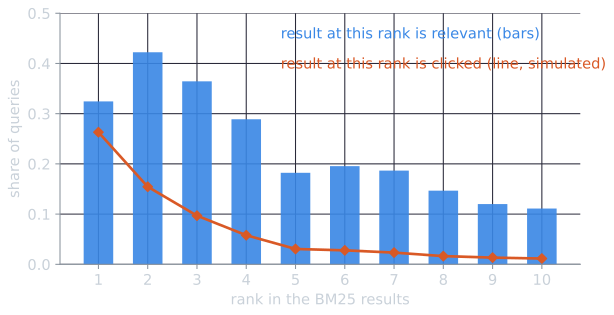
The fraction of relevant results falls by a factor of about four from rank 2 to rank 10, but simulated clicks fall by a factor of more than ten. (Rank 1 has fewer relevant results than rank 2 because, for 91 of the queries, BM25's first result is the document each query marks with the code −1, probably the paper the question was written from, which the judgments do not count as relevant; see test collections.) A raw click count would give the top result more than twenty times the clicks of the tenth, although the share of relevant results at the two ranks differs by a factor of three. Any metric built from clicks has to correct for the examination factor, either by modelling it or, as interleaving does, by arranging the experiment so that it affects both systems equally.
Interleaving
A/B tests compare groups of users, so differences between users add noise. Interleaving compares two rankings within a single user's results page. For each query, the rankings from systems A and B are merged into one list shown to the user, and clicks on results contributed by each system are credited to that system. Each impression is a direct comparison by the same user on the same query, which removes most of the variation between users.
In team-draft interleaving (Radlinski, Kurup, and Joachims, 2008), the merge works like picking teams. In each round a coin flip decides which system picks first. Each system then adds its highest-ranked result that is not already in the merged list, and that result is credited to the system's team. For example, with the rankings Chapelle et al. (2012) use to illustrate the method:
System A ranks:  a, b, c, d
System B ranks:  b, e, a, f
| Round | Coin flip | First pick | Second pick |
|---|---|---|---|
| 1 | A first | A adds a | B adds b |
| 2 | B first | B adds e | A adds c (its next result, b, is already shown) |
| 3 | A first | A adds d | B adds f (its next result, a, is already shown) |
The user sees a, b, e, c, d, f. If the user clicks b and e, both credited to B, then B wins this impression. Over many queries, the system that wins more impressions is preferred.
Because each comparison is made within one user's single interaction, interleaving is far more sensitive than an A/B test. Chapelle, Joachims, Radlinski, and Yue (2012) found that in most comparisons it needed one to two orders of magnitude fewer queries than click metrics measured on separate groups of users. Its limitation is that it gives only a preference between two rankers, not an absolute measurement of either. It also cannot compare changes that affect more than the ranking, such as a new page layout.
Every coin sequence
The coin flips are what make the method fair, and with three rounds there are only $2^3 = 8$ sequences, so they can all be listed (tools/experiments/online/online_examples.py). Subscripts show the team of each result:
| Coins (first picker in rounds 1, 2, 3) | Interleaved list |
|---|---|
| A A A | $a_A, b_B, c_A, e_B, d_A, f_B$ |
| A A B | $a_A, b_B, c_A, e_B, f_B, d_A$ |
| A B A | $a_A, b_B, e_B, c_A, d_A, f_B$ |
| A B B | $a_A, b_B, e_B, c_A, f_B, d_A$ |
| B A A | $b_B, a_A, c_A, e_B, d_A, f_B$ |
| B A B | $b_B, a_A, c_A, e_B, f_B, d_A$ |
| B B A | $b_B, a_A, e_B, c_A, d_A, f_B$ |
| B B B | $b_B, a_A, e_B, c_A, f_B, d_A$ |
Each list has probability 1/8. In this example the teams never change: a, c and d always belong to A, and b, e and f to B. Only the positions change. That is the point of the coins. Within each round, each team's pick is equally likely to be shown first, so neither team's results are systematically placed higher.
Credit then depends only on which results are clicked. Clicks on b and e make B win under all eight sequences; a click on a alone makes A win; clicks on a and e are a tie. A user who clicks one result at random from the top $k$, for any $k$, makes each system win with probability exactly 1/2. A user who ignores the content cannot create a preference, which Chapelle, Joachims, Radlinski, and Yue (2012, §3.2) give as the property that distinguishes team-draft from the older balanced interleaving.
Over an experiment, Chapelle et al. (2012, equation 4) summarize the outcomes as
$$\Delta_{AB} = \frac{\text{wins}(A) + \tfrac{1}{2}\,\text{ties}(A, B)}{\text{wins}(A) + \text{wins}(B) + \text{ties}(A, B)} - 0.5,$$
counting only impressions with at least one click. If A wins 40 percent of those impressions, B 30 percent, and 30 percent are ties, $\Delta_{AB} = 0.40 + 0.15 - 0.5 = 0.05$: A is preferred.
A case where team-draft errs
Fairness to a random user does not guarantee the right answer for real ones. Chapelle et al. (2012, §3.2) construct an ambiguous query: 49 percent of users want document a, 49 percent want b, and 2 percent want c, and each user clicks the first result that satisfies them. Ranking $R_1 = (a, b, \dots)$ satisfies 98 percent of users in its top two; $R_2 = (b, c, \dots)$ satisfies 51 percent. Enumerating the coin flips:
- If $R_1$ picks first, the list starts $a_1, b_2$: b goes to $R_2$, because $R_2$ picks it before $R_1$ reaches it.
- If $R_2$ picks first, it starts $b_2, a_1$.
Either way a is credited to $R_1$ and b and c to $R_2$. The 49 percent who want a vote for $R_1$, and the 49 percent who want b plus the 2 percent who want c vote for $R_2$, which wins 51 percent of the comparisons although it serves users far worse. The two rankings share a document that each would place in the top two, and the credit for it goes to whichever ranking claims it, not to the one that placed it best. The demo's third example reproduces this.
Where the sensitivity comes from
The same click simulation on Cranfield shows where the advantage comes from, and why its size varies. System A is BM25 with stemming and B is BM25 without it; on the judgments A is better (MAP 0.307 against 0.282). Each simulated impression is a random query and a user who clicks under the position model above. The A/B test sends half the impressions to each system and compares clicks per query with a t-test; interleaving shows every impression a team-draft list of the two top tens and tests whether A wins more impressions than B. For each design the script estimates the mean and variance of its per-impression statistic from 400,000 impressions, computes the impressions needed for 80 percent power at 0.05 with the formula from the A/B section, and then confirms by simulating experiments of that size (30 runs of 100 experiments; power came out between 0.78 and 0.81, and the false-positive rate with two identical systems at 0.04 to 0.05).
| Simulated users | A/B test | Interleaving | Ratio |
|---|---|---|---|
| All alike | 44,000 impressions (IQR 40,000 to 49,000) | 36,000 (33,000 to 41,000) | 1.2 |
| Differ in how much they click | 79,000 (71,000 to 94,000) | 29,000 (26,000 to 34,000) | 2.7 |
The figures are medians over 30 repetitions of the estimate, rounded to the nearest thousand, with interquartile ranges. In the first row the ranges overlap, so the advantage there is small and uncertain; in the second they are far apart.
In the second row each user's click probabilities are multiplied by a factor drawn from a gamma distribution with mean 1 and variance 2, so some users click on almost everything they examine and others on very little. This variation inflates the variance of clicks per query and nearly doubles the A/B test's requirement. Interleaving's requirement did not grow (it fell slightly), because a user who clicks a lot does so on both systems' results within the same list, and the comparison is made inside that list.
With identical users, interleaving gains little here, for a reason specific to these two systems: they return the same top document for 68 percent of queries, and when that shared document is clicked, the credit goes to whichever team the coin let claim it, adding noise rather than information. In 56 percent of impressions neither team won, either because the user clicked nothing or because the clicks split evenly. The size of interleaving's advantage therefore depends on how much users differ and on how different the two rankings are. Chapelle et al. (2012) found it to be one to two orders of magnitude in most comparisons on real search traffic. The simulation is not a substitute for that evidence; it shows the mechanism.
Evaluating from logs
Running a live experiment for every idea is slow, and showing users a bad ranking has a cost. Counterfactual evaluation estimates how a new ranker would have performed using logs collected while a different system was serving. This requires that the old system randomized some of what it showed. Li, Chu, Langford, and Wang (2011) evaluated news recommendation by replay: from logs collected while articles were chosen at random, keep only the events in which the logged choice matches what the new policy would have chosen, and average the outcomes of those events. More general estimators reweight each logged outcome by the inverse of the probability that the old system showed it. Click models, probabilistic models of how users scan and click, separate the effect of position from the effect of relevance. They can turn logged clicks into estimated relevance judgments or simulate user behavior for offline evaluation (Chuklin, Markov, and de Rijke, 2015).
Online and offline together
Online and offline evaluation answer different questions, and organizations that can run both use both. They do not always agree. User studies have found that improvements on batch measures do not always produce better performance on real search tasks (Hersh et al., 2000; Turpin and Hersh, 2001), the gap noted in relevance.
| Offline (test collections) | Online (live users) | |
|---|---|---|
| Measures | Agreement with relevance judgments | User behavior |
| Speed | Minutes, repeatable at will | Days or weeks |
| Cost of a bad system | None | Real users see it |
| Sensitivity | Depends on judgments and topic count | Very high with interleaving |
| Reproducibility | Exact | Low: users and content change |
| Available to | Anyone with the collection | Only operators of large services |
A common practice uses offline evaluation to screen ideas cheaply and safely, then confirms the promising ones online before deploying them. Disagreements between the two are informative. They reveal either judgments that do not reflect what users value or online metrics that do not measure what they were meant to. Research outside large companies relies almost entirely on offline evaluation, which is one reason test collections and the measures in this topic remain central to the field.
References
- Chapelle, O., Joachims, T., Radlinski, F., and Yue, Y. (2012). Large-scale validation and analysis of interleaved search evaluation. ACM Transactions on Information Systems, 30(1), article 6.
- Chuklin, A., Markov, I., and de Rijke, M. (2015). Click Models for Web Search. Morgan & Claypool.
- Fox, S., Karnawat, K., Mydland, M., Dumais, S., and White, T. (2005). Evaluating implicit measures to improve web search. ACM Transactions on Information Systems, 23(2), 147–168.
- Hersh, W., Turpin, A., Price, S., Chan, B., Kraemer, D., Sacherek, L., and Olson, D. (2000). Do batch and user evaluations give the same results? In Proceedings of SIGIR 2000, 17–24.
- Joachims, T., Granka, L., Pan, B., Hembrooke, H., and Gay, G. (2005). Accurately interpreting clickthrough data as implicit feedback. In Proceedings of SIGIR 2005, 154–161.
- Kohavi, R., Longbotham, R., Sommerfield, D., and Henne, R. M. (2009). Controlled experiments on the web: Survey and practical guide. Data Mining and Knowledge Discovery, 18(1), 140–181.
- Li, J., Huffman, S., and Tokuda, A. (2009). Good abandonment in mobile and PC internet search. In Proceedings of SIGIR 2009, 43–50.
- Li, L., Chu, W., Langford, J., and Wang, X. (2011). Unbiased offline evaluation of contextual-bandit-based news article recommendation algorithms. In Proceedings of WSDM 2011, 297–306.
- Radlinski, F., Kurup, M., and Joachims, T. (2008). How does clickthrough data reflect retrieval quality? In Proceedings of CIKM 2008, 43–52.
- Turpin, A. H., and Hersh, W. (2001). Why batch and user evaluations do not give the same results. In Proceedings of SIGIR 2001, 225–231.