System B has a mean average precision of 0.470 on ten topics, and system A has 0.434. Is B better? The answer depends on more than the two means. Average precision varies greatly from topic to topic: the same system may score 0.9 on an easy topic and 0.05 on a hard one, and the difference between two systems is usually much smaller than the difference between topics. A difference of 0.036 could be a real improvement, or it could be the result of which ten topics happened to be chosen. Significance testing is the standard way to decide, by asking how likely a difference this large would be if the two systems were really equally effective.
The course did not cover significance testing, but anyone comparing retrieval systems needs it. This article explains the reasoning, works five common tests on one small example where they disagree, applies them to a real comparison on the Cranfield collection where they agree, and then turns to how many topics an experiment needs and what goes wrong when many comparisons are made.
Topics are the unit
The comparison is between two systems run on the same topics, so the evidence is paired. For each topic there is one score for A and one for B, and the quantity of interest is the per-topic difference. Pairing removes the topic-to-topic variation, which dominates the raw scores, and leaves the system-to-system variation. Treating the two systems' scores as independent samples would bury a consistent difference under the variation between topics.
The example data, average precision on ten topics:
| Topic | 1 | 2 | 3 | 4 | 5 | 6 | 7 | 8 | 9 | 10 | Mean |
|---|---|---|---|---|---|---|---|---|---|---|---|
| System A | 0.42 | 0.31 | 0.55 | 0.28 | 0.61 | 0.47 | 0.35 | 0.52 | 0.39 | 0.44 | 0.434 |
| System B | 0.45 | 0.36 | 0.54 | 0.33 | 0.66 | 0.49 | 0.41 | 0.58 | 0.37 | 0.51 | 0.470 |
| B − A | 0.03 | 0.05 | −0.01 | 0.05 | 0.05 | 0.02 | 0.06 | 0.06 | −0.02 | 0.07 | 0.036 |
B is better on eight topics and worse on two, by small margins.
Each test starts from a null hypothesis, that the two systems are equally effective so the differences are only noise, and computes a p-value: the probability of a difference at least as large as the one observed if the null hypothesis were true. A small p-value, conventionally below 0.05, is taken as evidence that the difference is real.
The paired t-test
The paired t-test treats the differences $d_1, \dots, d_n$ as a sample from a normal distribution and asks whether its mean is zero. The test statistic is
$$t = \frac{\bar{d}}{s_d / \sqrt{n}},$$
where $\bar{d}$ is the mean difference and $s_d$ the standard deviation of the differences. Here $\bar{d} = 0.036$, $s_d = 0.0306$, and $n = 10$:
$$t = \frac{0.036}{0.0306 / \sqrt{10}} = 3.72,$$
with $n - 1 = 9$ degrees of freedom. The two-sided p-value is 0.005. Under the t-test, the improvement is significant.
The calculation step by step
Each step has a reason, so it is worth doing once by hand.
1. The mean difference. $\bar{d} = (0.03 + 0.05 - 0.01 + \dots + 0.07)/10 = 0.36/10 = 0.036$. This is the estimate of how much better B is.
2. How much the differences scatter. Each difference's deviation from the mean, and its square:
| Topic | 1 | 2 | 3 | 4 | 5 | 6 | 7 | 8 | 9 | 10 |
|---|---|---|---|---|---|---|---|---|---|---|
| $d_i$ | 0.03 | 0.05 | −0.01 | 0.05 | 0.05 | 0.02 | 0.06 | 0.06 | −0.02 | 0.07 |
| $d_i - \bar{d}$ | −0.006 | 0.014 | −0.046 | 0.014 | 0.014 | −0.016 | 0.024 | 0.024 | −0.056 | 0.034 |
| $(d_i - \bar{d})^2 \times 10^4$ | 0.36 | 1.96 | 21.16 | 1.96 | 1.96 | 2.56 | 5.76 | 5.76 | 31.36 | 11.56 |
The squares sum to $84.4 \times 10^{-4} = 0.00844$. The sample variance divides by $n - 1 = 9$ rather than 10, because the deviations are measured from $\bar{d}$, which was itself fitted to these ten numbers and so sits closer to them than the true mean would; dividing by 9 corrects that bias. So $s_d^2 = 0.00844/9 = 0.000938$ and $s_d = 0.0306$.
3. The standard error of the mean. A mean of $n$ independent differences varies less than one difference does, by a factor of $\sqrt{n}$: $s_d/\sqrt{10} = 0.0306/3.162 = 0.00968$. If the experiment were repeated on ten new topics, $\bar{d}$ would typically land about 0.01 away from where it landed this time.
4. The ratio. $t = 0.036/0.00968 = 3.72$: the observed mean is 3.7 standard errors from zero.
5. The reference distribution. If the true mean difference were zero and the differences normal, $t$ would follow Student's t distribution with 9 degrees of freedom. It has heavier tails than the normal distribution, because $s_d$ is itself an estimate from only ten numbers and is sometimes too small. For a two-sided test at 0.05 the critical value is 2.262 (against 1.96 for the normal), and the probability of $|t| \geq 3.72$ is 0.0048.
The same numbers give a 95% confidence interval for the true difference, $\bar{d} \pm 2.262 \times 0.00968 = [0.014, 0.058]$. The interval excludes zero exactly when the two-sided test is significant at 0.05, and it says more than the p-value: the data are consistent with an improvement as small as 0.014 or as large as 0.058.
The t-test assumes the differences are roughly normal. Per-topic differences in IR measures often are not, since they are bounded between −1 and 1 and sometimes dominated by a few topics. With fifty or more topics the test is fairly robust to this, but with few topics the assumption matters.
The sign test
The sign test ignores how large each difference is and counts only its direction. If the systems were equal, each topic would be equally likely to favor either system, so the number of topics favoring B would follow a binomial distribution with probability 1/2. B wins 8 of 10. The probability of 8 or more wins out of 10 by chance is $(\binom{10}{8} + \binom{10}{9} + \binom{10}{10})/2^{10} = 56/1024$, and doubling for a two-sided test gives $p = 0.109$. Under the sign test, the improvement is not significant.
The sign test makes no distributional assumption, but it discards the information in the sizes of the differences. A topic B wins by 0.07 counts the same as one it wins by 0.02. With few topics it has little power to detect real differences.
The Wilcoxon signed-rank test
The Wilcoxon signed-rank test sits between the sign test and the tests that use the raw differences. It replaces each difference by the rank of its absolute size, then gives the rank the difference's sign. The test statistic is the smaller of the two rank sums, the positive and the negative (Smucker, Allan, and Carterette, 2007, §2.2). Tied absolute values share the average of the ranks they span. Working in hundredths:
| Topic | 3 | 6 | 9 | 1 | 2 | 4 | 5 | 7 | 8 | 10 |
|---|---|---|---|---|---|---|---|---|---|---|
| $\lvert d_i \rvert \times 100$ | 1 | 2 | 2 | 3 | 5 | 5 | 5 | 6 | 6 | 7 |
| Rank | 1 | 2.5 | 2.5 | 4 | 6 | 6 | 6 | 8.5 | 8.5 | 10 |
| Sign | − | + | − | + | + | + | + | + | + | + |
The negative ranks are topic 3's 1 and topic 9's 2.5, so $W^- = 3.5$, and the positive ranks sum to $W^+ = 55 - 3.5 = 51.5$ (the ranks always total $n(n+1)/2 = 55$). Under the null hypothesis each rank is equally likely to carry either sign. Enumerating all $2^{10} = 1{,}024$ sign patterns, 12 give a smaller rank sum of 3.5 or less, so the exact two-sided p-value is $12/1024 = 0.012$.
The ranks keep the order of the magnitudes but not the magnitudes themselves: topic 10's difference of 0.07 counts 10, and topic 1's 0.03 counts 4, although one is more than twice the other. The test was devised in 1945 as a quick approximation that could be tabulated by hand (Smucker, Allan, and Carterette, 2007, §2.2). Its null distribution is the randomization distribution described next, applied to ranks instead of differences, and the sign test is the same thing applied to signs alone (§§2.2–2.3).
The randomization test
The randomization test, also called a permutation test, asks directly how unusual the observed difference would be if the labels "A" and "B" were arbitrary. If the systems were equivalent, then on each topic, swapping which score belongs to which system would be equally plausible, which flips the sign of that topic's difference. With 10 topics there are $2^{10} = 1{,}024$ ways to assign signs. For each, compute the mean difference, and count how many are at least as extreme as the observed 0.036. In this example, 14 of the 1,024 assignments are, so
$$p = \frac{14}{1024} = 0.014.$$
The improvement is significant, though less decisively than under the t-test. For larger topic sets, enumerating every assignment is infeasible, and a random sample of, say, 100,000 assignments is used instead:
import random


def randomization_test(a, b, trials=100_000, seed=0):
    """Two-sided paired randomization test on per-topic scores a and b."""
    rng = random.Random(seed)
    diffs = [y - x for x, y in zip(a, b)]
    observed = abs(sum(diffs) / len(diffs))
    extreme = 0
    for _ in range(trials):
        total = sum(d if rng.random() < 0.5 else -d for d in diffs)
        if abs(total / len(diffs)) >= observed - 1e-12:
            extreme += 1
    return extreme / trials
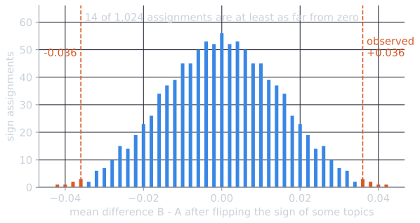
The 14 extreme assignments come in mirror pairs. The observed assignment itself is one, and flipping every sign gives its mirror image at −0.036. Six more reach at least +0.036. Making topic 3, topic 9, or both positive raises the mean to 0.038, 0.040, or 0.042. Three further patterns trade one of those gains for a loss elsewhere: topics 6 and 9 flipped (0.036), topics 3, 6 and 9 (0.038), and topics 1, 3 and 9 (0.036). Each of the seven has a mirror on the negative side, so the two-sided p-value is twice the one-sided $7/1024$.
A Monte Carlo p-value is itself an estimate. With 100,000 samples, 30 runs of the sampled test with different seeds gave a median of 0.0137 and an interquartile range of 0.0135 to 0.0140, around the exact 0.0137 (computed with numpy's generator in tools/experiments/cranfield/significance.py; the code above with seed 0 gives 0.0146). The sampling error, a few ten-thousandths, is negligible for deciding at 0.05 but should be kept in mind when a p-value is reported to four places.
What the test responds to. The randomization test looks at the consistency of a difference, not only its mean. Suppose the whole 0.36 of total improvement came from one topic: nine differences of zero and one of 0.36. The mean difference is the same 0.036. But now every sign assignment gives a mean of either +0.036 or −0.036, so all 1,024 are as extreme as the observed one, and $p = 1$. The t-test gives $p = 0.34$. One topic carrying the whole gain is no evidence that the next topic will show any gain, and both tests say so.
The bootstrap
The bootstrap takes a different route to the same question. It treats the ten topics as a sample from a population of possible topics and imitates drawing new samples by resampling the ten observed differences with replacement: a bootstrap sample of ten might contain topic 7 three times and topic 3 not at all. Repeating this many times, and computing the mean difference of each resample, gives the bootstrap distribution of the mean.
Two things are read from it:
- A confidence interval. The 2.5th and 97.5th percentiles of 100,000 resampled means are 0.017 and 0.053 (identical to three decimals over 30 seeds). This is the percentile interval, the bootstrap's counterpart of the t interval [0.014, 0.058], and here it is narrower.
- A p-value by the shift method (Smucker, Allan, and Carterette, 2007, §2.4). The bootstrap distribution is centred on the observed mean, not on zero. The shift method moves it to have mean zero, takes that as the null distribution, and counts the resampled means at least 0.036 from zero. Here that gives $p = 0.00016$ (median of 30 seeds; IQR 0.00014 to 0.00019), almost a hundred times smaller than the randomization test's 0.014.
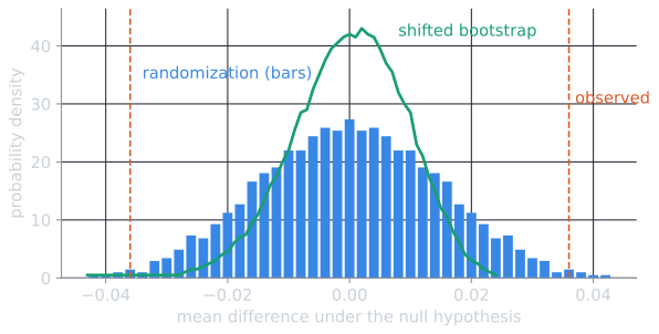
Why so different? The two null distributions have different spreads, and the difference can be computed exactly. Flipping signs at random gives each difference a mean of zero and a variance of $d_i^2$, so the randomization distribution of $\bar{d}$ has variance $\sum d_i^2 / n^2$. Resampling with replacement draws from the ten values with variance $\sum (d_i - \bar{d})^2 / n$, so the bootstrap mean has variance $\sum (d_i - \bar{d})^2 / n^2$. Since $\sum d_i^2 = \sum (d_i - \bar{d})^2 + n\bar{d}^2$, the randomization null is wider by exactly the term that the observed effect contributes:
$$\sqrt{0.0214}/10 = 0.0146 \quad \text{versus} \quad \sqrt{0.00844}/10 = 0.0092.$$
With a consistent effect and only ten topics, that term is a large part of the total, and the shifted bootstrap reports far more confidence than the data justify. With many topics and a small effect relative to the scatter, $n\bar{d}^2$ is small beside $\sum(d_i - \bar{d})^2$ and the two agree, which is what Smucker, Allan, and Carterette found on TREC runs of 50 topics. They also noted a small systematic tendency of the bootstrap toward smaller p-values (§4). The bootstrap is a large-sample method, and ten topics is not a large sample.
Why the tests disagree
| Test | Uses | p-value | Significant at 0.05? |
|---|---|---|---|
| Paired t-test | magnitudes, assumes normality | 0.005 | yes |
| Randomization test | magnitudes, exact | 0.014 | yes |
| Wilcoxon signed-rank | ranks of magnitudes | 0.012 | yes |
| Bootstrap, shift method | magnitudes, resampled | 0.0002 | yes |
| Sign test | directions only | 0.109 | no |
The tests use different information and make different assumptions. The sign test uses only directions. The t-test uses magnitudes and assumes normality. The randomization test uses magnitudes and assumes only that the labels are exchangeable under the null hypothesis. The Wilcoxon test uses the order of the magnitudes, and the bootstrap assumes the topics are a random sample from a population that the observed ten represent well. Smucker, Allan, and Carterette (2007) compared tests on TREC data and found that the t-test, the randomization test, and the bootstrap generally agreed with one another, while the sign test and the Wilcoxon signed-rank test often gave different answers. They recommended the randomization test, noted that the t-test led to the same conclusions on their data, and advised against the sign and Wilcoxon tests for comparing IR systems.
A real comparison: does stemming help on Cranfield?
The ten-topic example was built to make the tests disagree. On a real comparison with a reasonable number of topics they usually agree, and the reason for pairing becomes visible. The question is the one that opens test collections: does a stemmer improve retrieval? The two systems are BM25 ($k_1 = 1.2$, $b = 0.75$) with and without the Porter stemmer, run on all 225 Cranfield queries, scored by average precision (script tools/experiments/cranfield/significance.py).
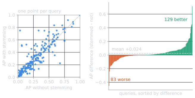
The left panel shows why pairing matters. Average precision ranges from near 0 to 1 across queries, with a standard deviation of about 0.23 for either system. The differences, in the right panel, have a standard deviation of 0.109, less than half as much, because a query that is hard for one system is hard for the other. The mean difference is 0.024 (MAP 0.307 against 0.282).
| Test | Statistic | Two-sided p |
|---|---|---|
| Paired t-test | $t = 0.0243/(0.1093/\sqrt{225}) = 3.34$, 224 df | 0.0010 |
| Randomization (20,000 samples, 30 seeds) | mean difference 0.0243 | 0.0007 (IQR 0.0006 to 0.0008) |
| Bootstrap, shift method (20,000 samples, 30 seeds) | mean difference 0.0243 | 0.0011 (IQR 0.0009 to 0.0012) |
| Wilcoxon signed-rank (13 zero differences dropped) | rank sums | 0.0003 |
| Sign test | 129 wins, 83 losses, 13 ties | 0.0019 |
| Unpaired t-test (wrongly ignoring the pairing) | $t = 1.11$ | 0.27 |
Every paired test finds the improvement significant, and the three that use the magnitudes agree closely, as Smucker, Allan, and Carterette (2007) found on TREC. The 95% intervals agree too: the t interval is [0.010, 0.039] and the bootstrap percentile interval [0.010, 0.039]. The last row is the mistake that pairing prevents. Treated as two independent samples of 225 scores, the same data give $p = 0.27$, because the comparison is then made against the scatter between queries, 0.23, instead of the scatter of the differences, 0.11.
The size of the effect, the mean difference divided by the standard deviation of the differences, is $0.0243/0.1093 = 0.22$. Unlike the p-value, it does not grow with the number of topics, and it determines how many topics are needed to see the difference reliably.
How many topics?
Fewer topics mean noisier comparisons. Voorhees and Buckley (2002) estimated, from TREC data, how often a conclusion that one system beats another would reverse on a different set of topics of the same size. With 50 topics, the conventional size of a TREC track, a difference in MAP had to be fairly large, several points in absolute terms, before the error rate became small. With 25 topics the required difference was larger still. Small topic sets can show a significant difference, as this example does, but small effects measured on them are fragile. Sakai (2016), reviewing a decade of papers in SIGIR and TOIS, found that many papers reported too little to assess their tests. Among those that could be assessed, some experiments were far too small to detect real differences, while others were so large that trivially small differences became significant. Sakai recommended reporting effect sizes alongside p-values and choosing sample sizes in advance from the effect sizes found in earlier studies.
Subsets of Cranfield
Cranfield's 225 queries allow a direct look at what smaller topic sets would have shown. For three comparisons with different true differences, the script draws random subsets of $n$ queries (300 subsets for each size, repeated over 30 seeds; medians reported) and asks two questions: how often does the subset show the opposite sign to the full set, and how often does a paired t-test on the subset find a significant difference in the right direction? The second is the power of the experiment.
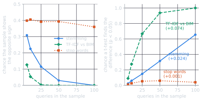
| Queries | Stemming: wrong sign | Stemming: detected | TF-IDF vs BIM: wrong sign | TF-IDF vs BIM: detected |
|---|---|---|---|---|
| 10 | 23% | 6% | 5% | 28% |
| 25 | 12% | 15% | 0.3% | 67% |
| 50 | 3% | 32% | 0% | 94% |
| 100 | 0% | 66% | 0% | 100% |
The stemming improvement is real (on all 225 queries, $p = 0.001$), yet an experiment with the conventional 50 topics would detect it only about one time in three. The subsets are drawn from a fixed pool of 225, so at 100 queries they share much of their content with the full set and the power is slightly overstated; for truly new topics the normal approximation below gives 60 percent at 100 rather than 66.
The power can be planned. A two-sided test at level $\alpha$ detects a true mean difference $\delta$ with probability $1 - \beta$ when $\delta$ is $z_{1-\alpha/2} + z_{1-\beta}$ standard errors from zero. The standard error is $s_d/\sqrt{n}$, so solving for $n$:
$$n \approx (z_{1-\alpha/2} + z_{1-\beta})^2 \left(\frac{s_d}{\delta}\right)^2.$$
For $\alpha = 0.05$ and 80% power, $(1.960 + 0.842)^2 = 7.85$. With the stemming numbers, $s_d/\delta = 0.1093/0.0243 = 4.49$, so $n \approx 7.85 \times 20.2 \approx 158$ topics (158.4 with the unrounded inputs). That is the calculation Sakai recommends making before an experiment, with $s_d$ and $\delta$ taken from earlier work; it says that a collection of 50 topics is too small for an effect of this size, whatever the p-value of a particular run turns out to be. The same formula, applied to users instead of topics, sizes online experiments.
Pitfalls
Multiple comparisons. Testing twenty variants against a baseline at the 0.05 level will, on average, find one "significant" difference even if none is real. When many comparisons are made, the threshold must be adjusted, for instance with the Bonferroni correction, which divides the significance level by the number of comparisons, or with methods designed for comparing many systems at once (Carterette, 2012).
The arithmetic is short. If none of $m$ variants truly differs from the baseline and the tests are independent, each avoids a false alarm with probability $0.95$, so the chance that at least one raises a false alarm, the family-wise error rate, is $1 - 0.95^m$: 0.40 for ten variants, 0.64 for twenty. The Bonferroni correction tests each variant at $0.05/m$. Since the probability that at least one of several events happens is never more than the sum of their probabilities, the family-wise rate is then at most $m \times 0.05/m = 0.05$, whether or not the tests are independent.
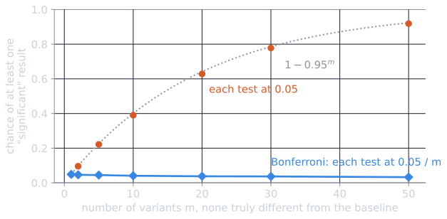
The simulation behind the figure builds variants that are truly no better than BM25: for each query, a variant's score differs from BM25's by the size of the real stemming difference on that query, with a random sign. Each variant is then compared with BM25 by a paired t-test on the 225 queries, 1,000 times for each $m$ and over 30 seeds. With twenty variants, at least one was "significant" in 63 percent of experiments (theory: 64 percent); with Bonferroni, in 3.8 percent. The price of the correction is power: a real improvement must now clear $0.05/20 = 0.0025$, which for the stemming effect needs about 300 topics rather than 158 by the formula above.
Statistical versus practical significance. With enough topics, a tiny difference becomes statistically significant without being worth anything to users. A p-value says whether a difference is likely real, not whether it matters. Reporting the size of the difference, ideally with a confidence interval, answers the second question.
Reusing the test set. A significance test assumes the test topics were not used to develop the system. Tuning on the test topics, discussed in test collections, invalidates the test however small the p-value.
Choosing the test after seeing the result. Running several tests and reporting the one that gives significance inflates the error rate just as multiple comparisons do. The test should be chosen in advance.
References
- Carterette, B. (2012). Multiple testing in statistical analysis of systems-based information retrieval experiments. ACM Transactions on Information Systems, 30(1), article 4.
- Sakai, T. (2016). Statistical significance, power, and sample sizes: A systematic review of SIGIR and TOIS, 2006–2015. In Proceedings of SIGIR 2016, 5–14.
- Smucker, M. D., Allan, J., and Carterette, B. (2007). A comparison of statistical significance tests for information retrieval evaluation. In Proceedings of CIKM 2007, 623–632.
- Voorhees, E. M., and Buckley, C. (2002). The effect of topic set size on retrieval experiment error. In Proceedings of SIGIR 2002, 316–323.