A query word in a document's title says more than the same word buried in its body. A paper with retrieval in its title is very likely about retrieval. One that mentions retrieval once on page twelve may not be. Documents have structure, such as titles, authors, abstracts, and dates, and a retrieval system can use that structure in two ways. It can let users search particular parts of a document, and it can score documents higher when the query matches more important parts. This article covers both, following Manning, Raghavan, and Schütze (2008, §6.1). It ends with the first example in the course of a scoring function whose parameters are learned from data rather than set by hand.
Fields and parametric search
Many documents carry metadata: structured attributes such as author, title, publication date, language, and format. Each attribute is a field with a limited set of values. Fields support parametric search, which restricts results by field values: articles by a particular author, published after 2020, in English. A digital library's advanced search form, with a box for each field, is the familiar interface.
A field is indexed separately from the text, in a structure suited to its values. Dates and numbers need range queries, so they are typically indexed in a search tree such as a B-tree, which can return every document dated between two values. A parametric query combined with a text query is evaluated as an intersection: the documents that satisfy the field conditions, intersected with those that match the text. This is the Boolean filtering that survives inside ranked search engines.
Zones
Zones are like fields, except that their content is free text: a title, an abstract, a section heading, the body. A query can be restricted to a zone, for example retrieval in the title. Zones can be indexed in two ways:
- Separate dictionaries. Build a separate inverted index for each zone, or equivalently qualify each term with its zone in a single dictionary:
william.author,william.title,william.body, each with its own postings list. - Zones in the postings. Keep one dictionary entry per term and record, in each posting, which zones of the document contain the term:
william → 2.author, 2.title, 3.author, 4.title, ....
The second encoding keeps the dictionary small and puts all of a term's zone information for a document in one place. That is exactly what a scoring function needs when it combines evidence from several zones (Manning, Raghavan, and Schütze, 2008, §6.1).
Weighted zone scoring
Weighted zone scoring assigns each of a document's $\ell$ zones a weight $g_1, \dots, g_\ell$, with each weight between 0 and 1 and the weights summing to 1. For a query $q$ and document $d$, let $s_i$ be 1 if the query matches zone $i$ of $d$ and 0 otherwise, where "matches" is defined by some Boolean condition, for example that the zone contains all the query terms. The score is
$$\text{score}(d, q) = \sum_{i=1}^{\ell} g_i \, s_i.$$
The score lies between 0 and 1. It is 1 when the query matches every zone and 0 when it matches none. Because each $s_i$ is a Boolean match, the method is sometimes called ranked Boolean retrieval: it ranks the documents that a Boolean query retrieves.
With three zones weighted author 0.2, title 0.3, and body 0.5, the example weights used by Manning, Raghavan, and Schütze, four documents would score:
| Document | Zones matching the query | Score |
|---|---|---|
| $d_1$ | title, body | 0.3 + 0.5 = 0.8 |
| $d_2$ | author | 0.2 |
| $d_3$ | body | 0.5 |
| $d_4$ | author, title, body | 0.2 + 0.3 + 0.5 = 1.0 |
The ranking is $d_4$, $d_1$, $d_3$, $d_2$. A match in the body counts for more than a match in the author field here because the weights say so. Choosing the weights is the hard part.
When a zone matches only if it contains all the query terms, the scores can be computed in one pass over the postings, by intersecting the query terms' postings document by document and adding $g_i$ for every zone in which all terms occur. This is a small extension of the merge algorithm when zones are encoded in the postings.
A traced example
Manning, Raghavan, and Schütze (2008, Figure 6.4) give this procedure as ZoneScore. Here it is applied to the two-word query william shakespeare, with the weights above and postings that record, for each document, the zones containing the term:
| Term | Postings: document (zones) |
|---|---|
| william | 1 (author, title), 2 (author), 3 (title, body), 4 (body), 5 (author, body) |
| shakespeare | 1 (title, body), 2 (author, body), 3 (title, body), 5 (body), 6 (title) |
The merge walks both lists in docID order. Documents 4 and 6 appear in only one list and are passed over. For each document in both, a zone matches when both terms occur in it:
| Document | Zones with william | Zones with shakespeare | Zones with both | Score |
|---|---|---|---|---|
| 1 | author, title | title, body | title | 0.3 |
| 2 | author | author, body | author | 0.2 |
| 3 | title, body | title, body | title, body | 0.3 + 0.5 = 0.8 |
| 5 | author, body | body | body | 0.5 |
The ranking is 3, 5, 1, 2. Document 1 contains both words, but never in the same zone except the title, so it collects only the title's weight; its william in the author field and shakespeare in the body are separate pieces of evidence that this scoring ignores. Document 2 has both words in the author field, perhaps a book by an author named William Shakespeare, and gets the author weight. Whether a match "in a zone" should require all the query terms, as here, or count terms separately, is a design choice, and the second option leads toward the term-weighted scores of the rest of this topic.
Learning the weights
Weights could be set by intuition, but they can also be learned from examples of relevance. This is a simple instance of machine-learned relevance, which the course meets again in learning to rank (Manning, Raghavan, and Schütze, 2008, §6.1.2).
Suppose there are two zones, title and body, so the score is
$$\text{score}(d, q) = g \cdot s_T(d, q) + (1 - g) \cdot s_B(d, q),$$
with a single weight $g$ to learn. The training data is a set of examples, each consisting of a query, a document, the two Boolean match values $s_T$ and $s_B$, and a human judgment $r$ that is 1 if the document is relevant to the query and 0 if not. A good $g$ makes the scores close to the judgments, so choose $g$ to minimize the total squared error
$$\varepsilon(g) = \sum_{\text{examples}} \big(r - \text{score}(d, q)\big)^2.$$
Deriving the optimal weight
Examples in which both zones match score $g + (1 - g) = 1$, and examples in which neither matches score 0. In both cases the score does not depend on $g$, so those examples do not affect the choice. Only two kinds of example matter:
- Title matches, body does not ($s_T = 1$, $s_B = 0$): the score is $g$. The error is $(1 - g)^2$ if the document is relevant and $g^2$ if it is not.
- Body matches, title does not ($s_T = 0$, $s_B = 1$): the score is $1 - g$. The error is $g^2$ if the document is relevant and $(1 - g)^2$ if it is not.
Let $n_{10r}$ and $n_{10n}$ count the relevant and nonrelevant examples of the first kind, and $n_{01r}$ and $n_{01n}$ those of the second. Grouping terms with the same error,
$$\varepsilon(g) = (n_{10r} + n_{01n})(1 - g)^2 + (n_{10n} + n_{01r})\, g^2 + \text{constant}.$$
The first group is the examples that would be scored perfectly by putting all the weight on the title, and the second those that would be scored perfectly by putting it all on the body. The error is a parabola in $g$, and the two groups pull its lowest point in opposite directions.
Setting the derivative to zero, $-2(n_{10r} + n_{01n})(1 - g) + 2(n_{10n} + n_{01r})\, g = 0$, and collecting the terms in $g$, $(n_{10r} + n_{01n} + n_{10n} + n_{01r})\, g = n_{10r} + n_{01n}$, gives
$$g = \frac{n_{10r} + n_{01n}}{n_{10r} + n_{10n} + n_{01r} + n_{01n}}.$$
The second derivative, $2(n_{10r} + n_{01n} + n_{10n} + n_{01r})$, is positive whenever there is at least one example in which the zones disagree, so this point is a minimum, not a maximum. It also lies between 0 and 1 automatically, since the numerator is part of the denominator. If the zones never disagree, the denominator is zero and the training data says nothing about $g$.
The formula can be read directly. The numerator counts the examples in which trusting the title gives the right answer: the title matched and the document was relevant, or only the body matched and the document was not. The denominator counts all examples in which the two zones disagree. The optimal weight on the title is the fraction of disagreements that the title gets right.
A worked example
Take ten training examples:
| $s_T$ | $s_B$ | Relevant? | Count |
|---|---|---|---|
| 1 | 1 | yes | 2 |
| 1 | 0 | yes | 2 |
| 1 | 0 | no | 1 |
| 0 | 1 | yes | 1 |
| 0 | 1 | no | 3 |
| 0 | 0 | no | 1 |
Here $n_{10r} = 2$, $n_{10n} = 1$, $n_{01r} = 1$, and $n_{01n} = 3$, so
$$g = \frac{2 + 3}{2 + 1 + 1 + 3} = \frac{5}{7} \approx 0.714.$$
Evaluating the error at several values of $g$ confirms the minimum:
| $g$ | 0 | 0.25 | 0.5 | 0.714 | 0.75 | 1 |
|---|---|---|---|---|---|---|
| $\varepsilon(g)$ | 5.000 | 2.938 | 1.750 | 1.429 | 1.438 | 2.000 |
In this training data, a title match is the more reliable signal, and the learned weight puts more than two-thirds of the score on it.
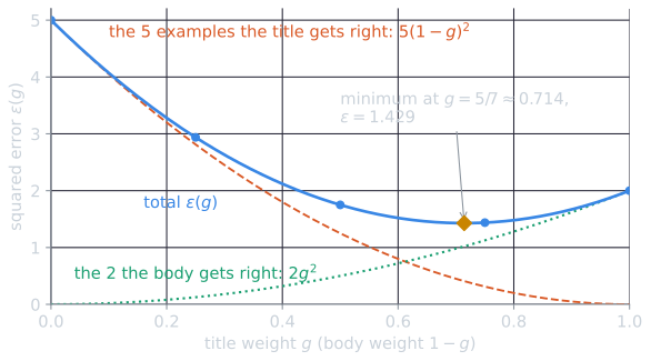
Here the constant is 0: the two examples in which both zones matched were relevant, and the one in which neither matched was not, so the score was exactly right for all three whatever $g$ is. With other data the constant can be positive, which raises the whole curve without moving its minimum.
What the learned weight means
With $g = 5/7$, the scoring function gives four possible scores, one for each pattern of matches:
| Title matches | Body matches | Score | Fraction relevant in training |
|---|---|---|---|
| yes | yes | 1 | 2 of 2 |
| yes | no | $g \approx 0.714$ | 2 of 3, 0.667 |
| no | yes | $1 - g \approx 0.286$ | 1 of 4, 0.250 |
| no | no | 0 | 0 of 1 |
Squared error is minimized, for any group of examples given the same score, by setting that score to the group's fraction of relevant examples. If the title-only and body-only scores could be chosen separately, least squares would set them to 0.667 and 0.250, the last column. They cannot, because both depend on the single weight $g$: title-only examples want $g = 0.667$, and body-only examples want $1 - g = 0.250$, that is, $g = 0.75$. The learned weight is the compromise, the average of the two wishes weighted by how many examples hold each: $(3 \times 0.667 + 4 \times 0.75) / 7 = 5/7$. This is the same formula as before, rewritten, and it shows what the scores approximate: the probability that a document with a given pattern of matches is relevant.
The same result as a regression
The derivation can be redone in a form that extends to any number of zones. Substitute $1 - g$ for the body weight and rearrange the error of one example:
$$r - \big(g\, s_T + (1 - g)\, s_B\big) = (r - s_B) - g\,(s_T - s_B).$$
With $x = s_T - s_B$ and $y = r - s_B$, this is $y - g x$, so minimizing the total squared error is fitting a straight line through the origin, $y = g x$, by least squares. The answer is the familiar $g = \sum x y / \sum x^2$. Examples in which the zones agree have $x = 0$ and drop out. A title-only example has $x = 1$ and $y = r$, and a body-only example has $x = -1$ and $y = r - 1$, so $\sum xy = n_{10r} + n_{01n}$ and $\sum x^2$ is the number of disagreements, which is the formula again. In the worked example, $\sum xy = 5$ and $\sum x^2 = 7$.
Three zones
With author, title and body zones, weights $g_A$, $g_T$ and $g_B = 1 - g_A - g_T$, the same substitution gives
$$r - s_B = g_A (s_A - s_B) + g_T (s_T - s_B) + \text{error},$$
a linear regression of $y = r - s_B$ on two variables $x_1 = s_A - s_B$ and $x_2 = s_T - s_B$, again through the origin. Take twenty training examples:
| $s_A$ | $s_T$ | $s_B$ | Relevant? | Count |
|---|---|---|---|---|
| 1 | 1 | 1 | yes | 2 |
| 0 | 1 | 1 | yes | 3 |
| 0 | 1 | 0 | yes | 2 |
| 0 | 1 | 0 | no | 1 |
| 0 | 0 | 1 | yes | 2 |
| 0 | 0 | 1 | no | 4 |
| 1 | 0 | 0 | yes | 1 |
| 1 | 0 | 0 | no | 2 |
| 1 | 0 | 1 | no | 1 |
| 0 | 0 | 0 | no | 2 |
The least-squares weights solve the normal equations $\left(\sum \vec{x}\,\vec{x}^{\mathsf{T}}\right) \vec{g} = \sum y\, \vec{x}$, sums taken over the examples with their counts:
$$\begin{pmatrix} 12 & 6 \\ 6 & 10 \end{pmatrix} \begin{pmatrix} g_A \\ g_T \end{pmatrix} = \begin{pmatrix} 5 \\ 7 \end{pmatrix}.$$
The determinant is $12 \times 10 - 6 \times 6 = 84$, so $g_A = (5 \times 10 - 6 \times 7)/84 = 2/21 \approx 0.095$ and $g_T = (12 \times 7 - 6 \times 5)/84 = 9/14 \approx 0.643$, which leaves $g_B = 11/42 \approx 0.262$. The total squared error is 3.024, against 3.900 for the weights 0.2, 0.3 and 0.5 used earlier and 3.778 for equal thirds. A search over a grid of all weight triples summing to 1, in steps of 0.005, finds the same minimum. In this data an author match is weak evidence of relevance (one relevant example of three when only the author matched), and the learned weights nearly ignore it.
Here the solution happened to fall inside the allowed region, with every weight between 0 and 1. With other data, unconstrained least squares can return a negative weight, and the weights must then be found by least squares subject to the constraints. The approach generalizes further. With features that are not Boolean, such as a TF-IDF score per zone, the same regression applies unchanged. Replacing the squared error with measures closer to ranking quality, and the linear combination with richer models, leads to modern learned ranking functions.
Zones in ranked models
Weighted zone scoring uses only whether each zone matches. The rest of this topic develops scores based on how often each term occurs and how informative it is, beginning with TF-IDF. The two ideas combine naturally. A score can be computed per zone with TF-IDF and the zone scores combined with weights. Or, as in BM25F (Robertson, Zaragoza, and Taylor, 2004), term frequencies from different zones can be weighted and summed before a single score is computed. Web search engines weight the title and the anchor text of incoming links separately from the body (see how a web search engine answers a query), and enterprise and product search engines commonly weight titles and other fields.
The worked examples are computed by tools/experiments/vsm/zones.py in the site repository, and the figure by tools/figures/zones-and-weighted-zone-scoring.py.
References
- Manning, C. D., Raghavan, P., and Schütze, H. (2008). Introduction to Information Retrieval, section 6.1. Cambridge University Press.
- Robertson, S., Zaragoza, H., and Taylor, M. (2004). Simple BM25 extension to multiple weighted fields. In Proceedings of CIKM 2004, 42–49.