For the query best car insurance, the words do not matter equally. Car and insurance say what the user wants, while best appears in so many documents, on every subject, that it does less to distinguish one from another. Within a single document, a word that appears ten times is probably more central than one that appears once. A ranking function needs to capture both observations: how important a term is within a document, and how informative the term is across the collection. TF-IDF weighting combines them, and its two components, term frequency and inverse document frequency, underlie most of the ranking functions in this course.
This article defines both components and their product, following Manning, Raghavan, and Schütze (2008, §6.2). The next article uses the resulting weights as the coordinates of document vectors, and variants of TF-IDF refines how each component is computed.
A running example
The articles in this topic share one small collection, so that each new idea can be seen changing the same numbers. It has four documents and the query best car insurance. Each document is shown by its term counts after text processing (lowercasing, stop-word removal, and folding plurals such as rates to rate):
- $d_1$, a headline about car insurance rates: car insurance rates.
- $d_2$, a car review that repeats car and never mentions insurance.
- $d_3$, a page about auto insurance that says auto where others say car.
- $d_4$, a longer page about car loans and their rates.
| Term | $d_1$ | $d_2$ | $d_3$ | $d_4$ | query |
|---|---|---|---|---|---|
| auto | 0 | 1 | 3 | 0 | 0 |
| best | 0 | 2 | 1 | 2 | 1 |
| car | 1 | 5 | 0 | 3 | 1 |
| insurance | 1 | 0 | 2 | 0 | 1 |
| loan | 0 | 0 | 0 | 4 | 0 |
| rate | 1 | 0 | 0 | 3 | 0 |
A reader looking for car insurance would want $d_1$ and $d_3$, and would not want $d_2$ or $d_4$. That judgment is the yardstick for every scoring function below. The table is the collection's term-document count matrix, with one row per term and one column per document.
Term frequency
The term frequency $\mathit{tf}_{t,d}$ is the number of times term $t$ occurs in document $d$. Representing a document by the term frequencies of its terms, and nothing else, is the bag-of-words model. Word order is discarded, so Mary is quicker than John and John is quicker than Mary have identical representations. That loss seems severe, but for judging what a document is about, which words occur and how often turns out to carry most of the information. Phrases and word order are handled separately, with positional indexes.
A first ranking function simply adds up the term frequencies of the query terms:
$$\text{score}(q, d) = \sum_{t \in q} \mathit{tf}_{t,d}.$$
On the running example, this overlap score reads the query rows of the count matrix and adds them:
| Document | best + car + insurance | Overlap score |
|---|---|---|
| $d_1$ | 0 + 1 + 1 | 2 |
| $d_2$ | 2 + 5 + 0 | 7 |
| $d_3$ | 1 + 0 + 2 | 3 |
| $d_4$ | 2 + 3 + 0 | 5 |
The ranking is $d_2$, $d_4$, $d_3$, $d_1$: the two documents the reader does not want come first. The overlap score has two flaws, and both show here. All terms count equally, so a match on a word that appears in nearly every document counts as much as a match on a word that appears in very few, although the rare word says far more about whether the document is on topic. And repetition counts without limit, so five occurrences of car outweigh a document that matches the whole query once.
Inverse document frequency
A term is informative when it is rare: it appears in few documents, so its presence distinguishes those documents from the rest. The document frequency $\mathit{df}_t$ is the number of documents containing $t$. For a collection of $N$ documents, the inverse document frequency is
$$\mathit{idf}_t = \log_{10} \frac{N}{\mathit{df}_t}.$$
A term in every document has $\mathit{idf} = \log 1 = 0$. A term in one document in a million has $\mathit{idf} = 6$. The logarithm compresses the range, so a term a thousand times rarer gets a weight 3 higher, not a thousand times higher. The base of the logarithm does not affect rankings, since changing it multiplies every weight by the same constant.
In the running example, $N = 4$, and the document frequencies are read off the count matrix by counting the nonzero entries in each row:
| Term | $\mathit{df}_t$ | $N / \mathit{df}_t$ | $\mathit{idf}_t$ |
|---|---|---|---|
| auto | 2 | 4/2 | 0.301 |
| best | 3 | 4/3 | 0.125 |
| car | 3 | 4/3 | 0.125 |
| insurance | 2 | 4/2 | 0.301 |
| loan | 1 | 4/1 | 0.602 |
| rate | 2 | 4/2 | 0.301 |
Insurance occurs in half the documents and car in three-quarters, so insurance gets the larger weight, 0.301 against 0.125. With only four documents the possible values are coarse, just 0, 0.125, 0.301 and 0.602, but the order is what matters.
Document frequency is used rather than collection frequency, the total number of occurrences, because it measures how widely a term is spread across documents, which is what discrimination depends on. As described in term statistics, try and insurance have nearly equal collection frequencies in Reuters, but insurance is concentrated in far fewer documents. It is the better discriminator, and only document frequency shows it. The running example shows the same thing on a small scale: auto and loan each occur 4 times in all, but loan is confined to one document and auto is spread over two, so loan gets the higher IDF.
Manning, Raghavan, and Schütze (2008, §6.2.1) give document frequencies from the Reuters RCV1 collection, which has $N = 806{,}791$ documents:
| Term | $\mathit{df}_t$ | $\mathit{idf}_t$ |
|---|---|---|
| auto | 6,723 | 2.08 |
| car | 18,165 | 1.65 |
| insurance | 19,241 | 1.62 |
| best | 25,235 | 1.50 |
The differences are modest because all four terms are moderately common. (The textbook's tables draw on different versions of the Reuters data, which is why insurance has a different document frequency here than in the comparison described in term statistics.) For a term such as the, present in nearly every document, the weight would be close to zero, and for a rare technical term it would be several times larger.
The shape of the IDF curve
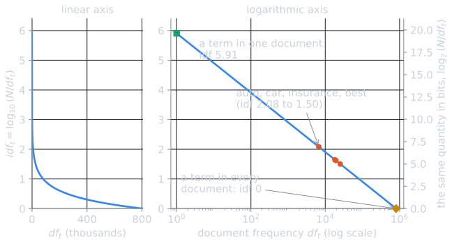
The left panel of the figure shows why the logarithm is there. Without it, $N/\mathit{df}_t$ would give a term in one document 806,791 times the weight of a term in every document, and one rare word in a query would swamp everything else. With it, the largest possible weight is $\log_{10} 806{,}791 \approx 5.91$. The right panel shows the same function against $\log \mathit{df}_t$, where it is a straight line of slope $-1$: $\mathit{idf}_t = \log N - \log \mathit{df}_t$. A term's weight depends only on how many powers of ten separate its document frequency from the collection size.
The idea originated with Karen Spärck Jones (1972), who showed experimentally that weighting terms by a decreasing function of how many documents they occur in improved retrieval. She presented this as a statistical interpretation of term specificity: a term's specificity is judged by how many documents it is used in, not by its meaning.
Combining them
The TF-IDF weight of term $t$ in document $d$ is the product
$$\text{tf-idf}_{t,d} = \mathit{tf}_{t,d} \times \mathit{idf}_t.$$
It is highest when a term occurs many times in a few documents, lower when it occurs fewer times or in more documents, and lowest, zero, when it occurs in every document. Replacing raw term frequency in the overlap score gives
$$\text{score}(q, d) = \sum_{t \in q} \text{tf-idf}_{t,d}.$$
The running example weighted
Multiplying each row of the count matrix by its term's IDF gives the TF-IDF matrix. Values are rounded to three decimals and computed from unrounded IDFs:
| Term | $d_1$ | $d_2$ | $d_3$ | $d_4$ |
|---|---|---|---|---|
| auto | 0 | 0.301 | 0.903 | 0 |
| best | 0 | 0.250 | 0.125 | 0.250 |
| car | 0.125 | 0.625 | 0 | 0.375 |
| insurance | 0.301 | 0 | 0.602 | 0 |
| loan | 0 | 0 | 0 | 2.408 |
| rate | 0.301 | 0 | 0 | 0.903 |
The score of each document adds its weights for the three query terms:
| Document | best + car + insurance | TF-IDF score |
|---|---|---|
| $d_1$ | 0 + 0.125 + 0.301 | 0.426 |
| $d_2$ | 0.250 + 0.625 + 0 | 0.875 |
| $d_3$ | 0.125 + 0 + 0.602 | 0.727 |
| $d_4$ | 0.250 + 0.375 + 0 | 0.625 |
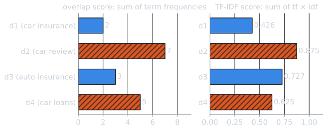
IDF has done part of the job. Insurance, the rarer and more specific query term, now counts for more than twice as much per occurrence as best or car, and the auto-insurance page $d_3$ rises from third to second. But $d_2$ is still first: five occurrences of car at 0.125 each outweigh anything $d_1$ can offer. And $d_1$, which matches two of the three query terms and is exactly what the reader wants, is last, because it is short and every count in it is 1. These are the two problems the rest of the topic fixes. Sublinear term frequency stops repetition from counting without limit, and the length normalization of cosine similarity stops long documents from collecting large scores merely by being long. With both, $d_1$ ranks first and $d_3$ second.
A worked example on Reuters statistics
Consider three documents with these term frequencies, from Exercise 6.10 of Manning, Raghavan, and Schütze (2008), weighted with the Reuters IDF values above:
| car | auto | insurance | best | |
|---|---|---|---|---|
| Doc 1 term frequency | 27 | 3 | 0 | 14 |
| Doc 2 term frequency | 4 | 33 | 33 | 0 |
| Doc 3 term frequency | 24 | 0 | 29 | 17 |
| Doc 1 TF-IDF | 44.55 | 6.24 | 0 | 21.00 |
| Doc 2 TF-IDF | 6.60 | 68.64 | 53.46 | 0 |
| Doc 3 TF-IDF | 39.60 | 0 | 46.98 | 25.50 |
For the query car insurance, the scores are Doc 1: 44.55, Doc 2: 60.06, and Doc 3: 86.58. Doc 3 ranks first, as it should: it uses both terms heavily. But Doc 1 scores 44.55 without containing insurance at all, purely because car appears 27 times. Raw term frequency lets one heavily repeated term carry a document a long way. That weakness motivates the sublinear scaling of term frequency. Longer documents also tend to have larger term frequencies, which motivates the length normalization of the next article.
IDF and single-term queries
IDF affects ranking only when a query has more than one term. For a query of one term, every document's score is multiplied by the same IDF value, so the order is unchanged. In the running example, the query car scores the documents 0.125, 0.625, 0 and 0.375, which is 0.125 times their counts of car, 1, 5, 0 and 3, and ranks them exactly as the counts do. IDF matters when it decides how much each query term contributes relative to the others. In best car insurance, it ensures that a match on insurance counts for more than a match on best.
Points that are easy to confuse
- TF belongs to a term in a document; IDF belongs to a term in a collection. A term has one IDF, shared by every document, and a TF-IDF weight for every document. Adding a document to the collection can change the IDF, and so the weights, of terms in documents that were not touched.
- IDF is not a stop list. A term in every document gets weight zero, which acts like removing it, but a common term that misses a few documents keeps a small positive weight. In the running example best is in three of the four documents and still counts 0.125 per occurrence.
- The query side and the document side are separate choices. The score above weights documents by TF-IDF and counts each query term once. Other schemes put IDF only on the query side, or on both. Variants of TF-IDF names these choices.
- "TF-IDF" names a family. Libraries differ in the base of the logarithm, in smoothing (for example $\log \frac{1 + N}{1 + \mathit{df}_t} + 1$), and in whether term frequency is dampened, so two implementations can give different numbers for the same data. The ideas are the same.
Why IDF works
IDF was introduced as an empirical observation, and several later arguments have tried to explain why it works. Robertson (2004) reviews them:
- Information theory. If a term occurs in a fraction $\mathit{df}_t / N$ of documents, then $\log(N/\mathit{df}_t)$ is the information, in the sense of Shannon, gained on learning that a document contains it. Rare terms are surprising and therefore informative. Robertson finds justifications along these lines problematic, and regards the probabilistic argument as the sounder one.
- Probability of relevance. The Binary Independence Model derives a term weight from the probabilities that a term appears in relevant and nonrelevant documents. When nothing is known about which documents are relevant, the weight reduces to approximately $\log(N/\mathit{df}_t)$. IDF is what the probabilistic model prescribes in the absence of relevance information.
- Discrimination. A term that occurs in nearly every document divides the collection into one large group and a few exceptions, which does little to separate relevant from nonrelevant documents. A term in few documents divides it sharply.
The information-theoretic reading, worked
Pick a document at random from Reuters. The probability that it contains car is $18{,}165 / 806{,}791 \approx 0.0225$. Learning that it does is a moderately surprising event, and Shannon's measure of the surprise, $-\log_2 0.0225$, is 5.47 bits. That is the IDF of car measured in bits instead of powers of ten: $1.648 \times \log_2 10 \approx 5.47$. The right-hand axis of the IDF figure gives every term's weight in these units.
The reading also explains why IDFs are added. If occurrences of different terms were independent, the probability that a random document contains both car and insurance would be the product $0.0225 \times 0.0238 \approx 0.000537$, and the information in that joint event would be the sum $1.648 + 1.623 = 3.270$ in base 10, since the logarithm turns the product into a sum. Summing IDFs over the matched query terms therefore ranks a document by how improbable its pattern of matches would be by chance. The weak points are the independence assumption, which is plainly false for car and insurance, and the fact that the argument says nothing about relevance. The probabilistic reading below starts from relevance instead.
The probabilistic reading, in one line
The Binary Independence Model, without relevance information, gives each matching term the weight $\log \frac{N - \mathit{df}_t}{\mathit{df}_t}$ (the derivation is in its article). For rare terms the $-\mathit{df}_t$ in the numerator hardly matters: for car in Reuters the two weights are 1.638 and 1.648. They part company for common terms. A term in half the documents gets IDF $\log 2 \approx 0.301$, but probabilistic weight $\log 1 = 0$, and a term in more than half gets a negative probabilistic weight, which practical systems clip at zero. This clipped form is the "probabilistic IDF" option of the SMART notation in variants of TF-IDF.
These arguments, the probabilistic one above all, suggest why TF-IDF works: it approximates quantities that more principled models derive, which is one reason it has lasted. Its components survive, in refined forms, in BM25 and in many features used by learned rankers.
Every number in the running example is computed by tools/experiments/vsm/running_example.py in the site repository, and the figures by tools/figures/tf-idf.py.
References
- Manning, C. D., Raghavan, P., and Schütze, H. (2008). Introduction to Information Retrieval, sections 6.2 and 6.4. Cambridge University Press.
- Robertson, S. (2004). Understanding inverse document frequency: On theoretical arguments for IDF. Journal of Documentation, 60(5), 503–520.
- Spärck Jones, K. (1972). A statistical interpretation of term specificity and its application in retrieval. Journal of Documentation, 28(1), 11–21.