Which of Shakespeare's plays contain the words Brutus and Caesar but not Calpurnia? Manning, Raghavan, and Schütze (2008, §1.1) open their textbook with this question because it shows why retrieval needs an index. For one person with a computer and the complete works, the obvious method is to scan the text of every play, the way the Unix tool grep does. That works for a few megabytes. It does not work for a billion documents, it does not work when thousands of queries arrive every second, and it gives no help with queries such as Romans within a few words of countrymen, or with ranking the results.
The alternative is to process the collection once, in advance, into a structure that answers such questions without reading the text again. This article builds that structure in two stages, first the incidence matrix, which is simple and does not scale, then the inverted index, which scales and is used by almost every search engine. The architecture article introduced the inverted index on four sentences. Here it is constructed systematically.
The term-document incidence matrix
The simplest index records, for every term and every document, whether the term occurs in the document. Arranged with terms as rows and documents as columns, this is the term-document incidence matrix. Part of the matrix for six of Shakespeare's plays (Manning, Raghavan, and Schütze, 2008, §1.1):
| Antony and Cleopatra | Julius Caesar | The Tempest | Hamlet | Othello | Macbeth | |
|---|---|---|---|---|---|---|
| Antony | 1 | 1 | 0 | 0 | 0 | 1 |
| Brutus | 1 | 1 | 0 | 1 | 0 | 0 |
| Caesar | 1 | 1 | 0 | 1 | 1 | 1 |
| Calpurnia | 0 | 1 | 0 | 0 | 0 | 0 |
| Cleopatra | 1 | 0 | 0 | 0 | 0 | 0 |
| mercy | 1 | 0 | 1 | 1 | 1 | 1 |
| worser | 1 | 0 | 1 | 1 | 1 | 0 |
Each row is a bit vector saying which documents contain a term, and each column is a bit vector saying which terms a document contains. A Boolean query becomes bitwise operations on rows, so the question about Brutus, Caesar, and Calpurnia can be answered without touching the text. The Boolean retrieval model works through that computation.
The matrix fails on size. Consider a modest collection of $N = 1$ million documents, each about 1,000 words long, with a vocabulary of $M = 500{,}000$ distinct terms. The matrix has
$$M \times N = 500{,}000 \times 1{,}000{,}000 = 5 \times 10^{11}$$
cells, half a trillion. But the collection contains only about $10^{9}$ tokens in total, so at most $10^{9}$ cells can contain a 1, and fewer still, since repeated words in a document share a cell. At least 99.8 percent of the matrix is zeros. The matrix is extremely sparse, and Zipf's law describes how the 1s are spread: most terms are rare, so most rows are almost entirely empty. Storing it explicitly wastes nearly all of its space recording what is not there.
A real collection shows the same proportions. Reuters-21578 (Lewis, 1997), a set of 10,788 news stories from 1987, has 29,187 distinct terms when its text is lowercased and split into runs of letters, as in the term statistics article. Its incidence matrix has $29{,}187 \times 10{,}788 = 314{,}869{,}356$ cells, of which only 725,793 contain a 1: 0.23 percent. Even at one bit per cell, the matrix takes 39.4 megabytes. Listing the 725,793 (term, document) pairs instead, as 4-byte document numbers, takes 2.9 megabytes, about a thirteenth as much, and the compression article shrinks that list to well under one megabyte. More than half of the terms (59 percent) occur in only one or two stories, so more than half of the matrix's rows hold at most two 1s among 10,788 cells.
The inverted index
The solution is to store only the 1s. For each term, record the list of documents that contain it. That is the inverted index, so called because it inverts the natural organization of a collection: a document lists the terms it contains, and the index lists, for each term, the documents that contain it.
The index has two parts:
- The dictionary, also called the vocabulary or lexicon, contains every term. For each term it stores the document frequency $\mathit{df}_t$, the number of documents containing it, and a pointer to its postings list.
- The postings lists, one per term, contain the identifiers of the documents in which the term occurs. Each entry is a posting. Together the lists form the postings file.
Each document is identified by a document identifier (docID), usually an integer assigned in the order documents are indexed. Postings lists are kept sorted by docID. Sorting is what makes Boolean queries efficient. Two sorted lists can be intersected in a single pass, advancing through both at once, in time proportional to their combined length, which is the merge algorithm developed in intersecting postings lists.
Building an index by sorting
The basic construction method has four steps (Manning, Raghavan, and Schütze, 2008, §1.2):
- Collect the documents to be indexed.
- Tokenize each document.
- Apply linguistic preprocessing (stop words, normalization, stemming) to produce index terms.
- Index the documents: produce a list of (term, docID) pairs, sort it, and group it into a dictionary and postings.
Take a small collection, from the exercises in chapter 1 of the same textbook:
| docID | Text |
|---|---|
| 1 | New home sales top forecasts |
| 2 | Home sales rise in July |
| 3 | Increase in home sales in July |
| 4 | July new home sales rise |
After lowercasing, removing in, and stemming with the original Porter algorithm, the documents produce these (term, docID) pairs, in document order:
(new,1) (home,1) (sale,1) (top,1) (forecast,1)
(home,2) (sale,2) (rise,2) (juli,2)
(increas,3) (home,3) (sale,3) (juli,3)
(juli,4) (new,4) (home,4) (sale,4) (rise,4)
(July stems to juli because the Porter stemmer turns a final y after a consonant into i, and increase loses its final e. See the Porter stemmer.) Sorting the pairs by term, then by docID, brings all occurrences of each term together, in docID order:
(forecast,1) (home,1) (home,2) (home,3) (home,4) (increas,3)
(juli,2) (juli,3) (juli,4) (new,1) (new,4) (rise,2) (rise,4)
(sale,1) (sale,2) (sale,3) (sale,4) (top,1)
Grouping consecutive pairs with the same term, and merging repeated pairs from the same document, gives the index:
| Term | $\mathit{df}$ | Postings |
|---|---|---|
| forecast | 1 | 1 |
| home | 4 | 1, 2, 3, 4 |
| increas | 1 | 3 |
| juli | 3 | 2, 3, 4 |
| new | 2 | 1, 4 |
| rise | 2 | 2, 4 |
| sale | 4 | 1, 2, 3, 4 |
| top | 1 | 1 |
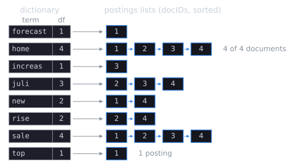
The query new AND rise intersects the lists for new (1, 4) and rise (2, 4) and returns document 4.
Three things in this construction are easy to miss. First, the document frequency in the dictionary is just the length of the postings list. It is stored separately because query processing and term weighting need it before, or instead of, reading the list. Second, the sort does the real work: after it, grouping is a single pass that compares each pair with the one before it. Third, the merging of repeated pairs is where information can be lost. Had the documents repeated a word, say sales twice in document 1, the pair (sale, 1) would appear twice before merging, and a docID-only index would keep no record of it. Keeping the count is the difference between the first two rows of the table in the section on postings.
Sorting is the expensive step. For a collection whose pairs fit in memory, it is a single in-memory sort. For one whose pairs do not, it must be done in blocks and merged, which is the subject of index construction.
Storing the dictionary
The dictionary is consulted for every query term, so it must support fast lookup. There are two main choices (Manning, Raghavan, and Schütze, 2008, §3.1):
- A hash table maps each term directly to its entry, giving lookup in constant expected time. It cannot find terms by prefix, since similar terms hash to unrelated positions, and it must be rebuilt or resized as the vocabulary grows.
- A search tree, usually a B-tree in disk-based systems, keeps terms in sorted order. Lookup takes logarithmic time, and the tree supports prefix and range queries, such as all terms beginning with auto, which spelling correction and wildcard queries need.
Large systems often use a sorted array of terms, searched by binary search and stored compactly, as described in index compression. In the example, the eight terms sorted are forecast, home, increas, juli, new, rise, sale, top, at positions 0 to 7. Looking up rise:
| Step | Range searched | Middle position | Term there | Comparison |
|---|---|---|---|---|
| 1 | 0 to 7 | 3 | juli | rise is later, so search 4 to 7 |
| 2 | 4 to 7 | 5 | rise | found |
Looking up retail, which is not in the dictionary, takes one more step: after position 5 (rise, later than retail) the range shrinks to position 4 (new, earlier), and then to nothing, so the search ends with the information that retail would sit between new and rise. That last fact is what a hash table cannot provide. It is enough to find every term with a given prefix, since they are stored together starting at the place the search ends. A dictionary of $M$ terms needs about $\log_2 M$ comparisons, 15 for the 29,187 terms of Reuters-21578 and 19 for 400,000. Since the dictionary is much smaller than the postings, it can usually be kept in memory even when the postings cannot.
Storing the postings
Postings lists vary enormously in length, from a single document for most terms to nearly every document for the most common ones. Two in-memory representations are common: linked lists, which make insertion cheap, and variable-length arrays, which use less space and are faster to scan because their contents are contiguous in memory (Manning, Raghavan, and Schütze, 2008, §1.2). In a simple static index on disk, each term's postings are stored as one contiguous run, so that a query reads each list sequentially. Indexes that are updated or compressed in blocks may split a list across several segments or blocks.
A posting can carry more than a docID, and what it carries determines what the system can do. The architecture article showed how each ranking model depends on particular statistics. In summary:
| Posting contents | Enables |
|---|---|
| docID only | Boolean retrieval |
| docID and term frequency | Weighted ranking such as TF-IDF and BM25 |
| docID, term frequency, and positions | Phrase and proximity queries, through a positional index |
| Any of the above, separated by field | Searching or weighting titles, headings, or anchor text separately |
In the four-document example, the postings of home and sale in each form look like this, with positions counted over all the words of a document, including the removed in, so that the original word distances are kept:
| Term | docIDs | docID: tf | docID: positions |
|---|---|---|---|
| home | 1, 2, 3, 4 | 1:1, 2:1, 3:1, 4:1 | 1:⟨2⟩, 2:⟨1⟩, 3:⟨3⟩, 4:⟨3⟩ |
| sale | 1, 2, 3, 4 | 1:1, 2:1, 3:1, 4:1 | 1:⟨3⟩, 2:⟨2⟩, 3:⟨4⟩, 4:⟨4⟩ |
The docID lists alone say that both words occur in every document, which answers home AND sale but cannot distinguish the phrase home sales from a document that mentions homes in one sentence and sales in another. The positions can: in every document the position of sale is one more than that of home, so all four documents contain the phrase. The positional index article develops the merge that checks this. Each richer form costs space. On Reuters-21578 the docID-only index has 725,793 postings, while a positional index must also store a position for each of the collection's 1,330,267 tokens, before any stop words are removed.
Collection-level statistics live elsewhere: the dictionary stores each term's document frequency, and a separate table stores each document's length and any document-level scores. Many systems also keep a forward index, mapping each document to its terms, or a copy of the document text, for generating snippets and computing features that depend on the whole document.
Why the inverted index won
Other structures have been proposed for text search, notably signature files, which store a compact bit pattern for each document, and suffix arrays, which index every position in the text. After a careful comparison, Zobel, Moffat, and Ramamohanarao (1998) concluded that inverted files were faster, smaller, and more flexible than signature files for the text-indexing workloads they studied. Suffix arrays support arbitrary substring search, but they are large and hard to update. The inverted index is space-efficient because it stores only what occurs, and it is query-efficient because a query reads only the postings of its own terms. It also extends naturally to everything retrieval needs: frequencies, positions, fields, and compression. The next two articles cover how to build one for a collection too large for memory and how to make it small.
References
- Lewis, D. D. (1997). Reuters-21578 text categorization test collection, distribution 1.0.
- Manning, C. D., Raghavan, P., and Schütze, H. (2008). Introduction to Information Retrieval, sections 1.1–1.2 and 3.1. Cambridge University Press.
- Zobel, J., and Moffat, A. (2006). Inverted files for text search engines. ACM Computing Surveys, 38(2), article 6.
- Zobel, J., Moffat, A., and Ramamohanarao, K. (1998). Inverted files versus signature files for text indexing. ACM Transactions on Database Systems, 23(4), 453–490.