Take a document and append a copy of it to itself. The new document says exactly the same things, in the same proportions, but every term frequency has doubled. A measure of similarity that treats the two as very different has missed the point. Yet if documents are points in space, with term frequencies as coordinates, the doubled document lies twice as far from the origin, and its distance from any query changes. Measuring the angle between vectors rather than the distance between points makes the two documents identical, because doubling a vector does not change its direction. That is the core idea of cosine similarity, the measure the vector space model (Salton, Wong, and Yang, 1975) uses to compare documents with queries and with one another.
This article sets up the vector representation, defines cosine similarity, and works through comparisons adapting examples from Manning, Raghavan, and Schütze (2008, §6.3). How to compute it efficiently for a whole collection is the subject of computing vector scores.
Documents as vectors
Fix a vocabulary of $M$ terms. A document $d$ becomes a vector $\vec{V}(d)$ with one component per term, where the component for term $t$ is a weight, typically the TF-IDF weight of $t$ in $d$, and 0 if $t$ does not occur. A collection of $N$ documents is then an $M \times N$ term-document matrix, with one column per document. The matrix is very sparse, since each document contains a tiny fraction of the vocabulary. A search engine does not store it as a matrix; the inverted index stores the same nonzero entries, organized by row.
A query is treated the same way. The query jealous gossip is a vector with nonzero components for jealous and gossip and zeros elsewhere. Representing queries and documents in the same space is what makes it possible to compare them with a single measure.
In the four-document running example introduced in TF-IDF weighting, the vocabulary has six terms (auto, best, car, insurance, loan, rate), so every document and the query best car insurance are vectors in a six-dimensional space. The columns of the TF-IDF matrix in that article are the document vectors. The car-insurance headline $d_1$, for example, is $(0, 0, 0.125, 0.301, 0, 0.301)$.
Angle, not distance
The natural measure of difference between two points is the Euclidean distance. For a query and a document it gives the wrong answer, for the reason in the opening paragraph. Consider two terms, a query $q = (1, 1)$, a document $d = (3, 1)$, and the doubled document $d' = (6, 2)$:
| Euclidean distance from $q$ | Cosine similarity with $q$ | |
|---|---|---|
| $d = (3, 1)$ | 2.00 | 0.894 |
| $d' = (6, 2)$ | 5.10 | 0.894 |
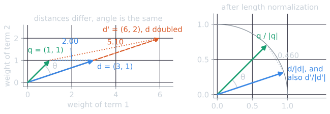
By distance, the doubled document is much less similar to the query, simply because it is longer. By angle, the two are identical. Since long documents have larger term frequencies whether or not they are more relevant, distance would systematically penalize them for their length. The angle depends only on the proportions among the terms.
The penalty also runs the other way: distance rewards documents for being short. A query vector is short, since it has a few small weights, so any document near the origin is close to it, whether or not it shares a term. An empty document, the zero vector, is at distance $\lvert \vec{q} \rvert$ from every query. The running example below shows that this is not a curiosity.
The cosine measure
The dot product of two vectors is the sum of the products of their components,
$$\vec{V}(d_1) \cdot \vec{V}(d_2) = \sum_{t} V_t(d_1)\, V_t(d_2),$$
which is large when the two vectors give large weights to the same terms. It also grows with the vectors' lengths. Dividing by both lengths gives the cosine of the angle $\theta$ between them:
$$\text{sim}(d_1, d_2) = \cos\theta = \frac{\vec{V}(d_1) \cdot \vec{V}(d_2)}{\lvert \vec{V}(d_1) \rvert \, \lvert \vec{V}(d_2) \rvert},$$
where $\lvert \vec{V} \rvert = \sqrt{\sum_t V_t^2}$ is the Euclidean length. With non-negative weights, the cosine ranges from 0, when the vectors share no terms and are at right angles, to 1, when they point in the same direction.
Why is this ratio the cosine of an angle? In two dimensions, write each vector by its length and direction, $\vec{a} = \lvert \vec{a} \rvert (\cos\alpha, \sin\alpha)$ and $\vec{b} = \lvert \vec{b} \rvert (\cos\beta, \sin\beta)$. Then $\vec{a} \cdot \vec{b} = \lvert \vec{a} \rvert \lvert \vec{b} \rvert (\cos\alpha \cos\beta + \sin\alpha \sin\beta) = \lvert \vec{a} \rvert \lvert \vec{b} \rvert \cos(\alpha - \beta)$, by the angle-difference identity, and $\alpha - \beta$ is the angle between them. Any two vectors, in any number of dimensions, lie in a common plane through the origin, so the same holds in the $M$-dimensional term space. For the figure's example, $q \cdot d = 1 \times 3 + 1 \times 1 = 4$, $\lvert q \rvert = \sqrt{2}$, $\lvert d \rvert = \sqrt{10}$, and $\cos\theta = 4 / \sqrt{20} \approx 0.894$, an angle of about 26.6 degrees. For $d'$ the dot product doubles to 8 and the length doubles to $\sqrt{40}$, so the ratio does not change.
The division is length normalization. It is often done once, in advance, by scaling every vector to length 1. For unit vectors $\vec{v}(d) = \vec{V}(d) / \lvert \vec{V}(d) \rvert$, the cosine is simply the dot product, $\text{sim}(d_1, d_2) = \vec{v}(d_1) \cdot \vec{v}(d_2)$. Search engines store each document's length, or its normalized weights, at indexing time, so that query-time scoring only needs to multiply and add.
Angle and distance after normalization
Normalization also connects angle and distance. For unit vectors $\vec{v}_1$ and $\vec{v}_2$, expand the squared distance as a dot product of the difference with itself:
$$\lvert \vec{v}_1 - \vec{v}_2 \rvert^2 = (\vec{v}_1 - \vec{v}_2) \cdot (\vec{v}_1 - \vec{v}_2) = \vec{v}_1 \cdot \vec{v}_1 - 2\, \vec{v}_1 \cdot \vec{v}_2 + \vec{v}_2 \cdot \vec{v}_2.$$
Each vector has length 1, so $\vec{v}_1 \cdot \vec{v}_1 = \vec{v}_2 \cdot \vec{v}_2 = 1$, and $\vec{v}_1 \cdot \vec{v}_2 = \cos\theta$. Hence
$$\lvert \vec{v}_1 - \vec{v}_2 \rvert^2 = 2(1 - \cos\theta).$$
The right-hand side decreases as $\cos\theta$ increases, so ranking by cosine is the same as ranking by Euclidean distance between the normalized vectors. In the figure, $\sqrt{2(1 - 0.894)} \approx 0.460$, the chord between the two points on the unit circle. The problem with distance was never distance itself, but distance between vectors of different lengths.
The running example scored
Score the running example's documents against best car insurance, with TF-IDF weights on both sides and cosine normalization of both, the scheme called ntc.ntc in the SMART notation. The query's TF-IDF vector has weights 0.125 for best and car and 0.301 for insurance, and length $\sqrt{0.125^2 + 0.125^2 + 0.301^2} \approx 0.349$. Each document's length is the square root of the sum of its squared TF-IDF weights. For $d_1$ that is $\sqrt{0.125^2 + 0.301^2 + 0.301^2} \approx 0.444$.
| Document | Dot product with query | Length | Cosine |
|---|---|---|---|
| $d_1$ | 0.125 × 0.125 + 0.301 × 0.301 = 0.106 | 0.444 | 0.106 / (0.444 × 0.349) = 0.686 |
| $d_2$ | 0.250 × 0.125 + 0.625 × 0.125 = 0.109 | 0.737 | 0.425 |
| $d_3$ | 0.125 × 0.125 + 0.602 × 0.301 = 0.197 | 1.093 | 0.516 |
| $d_4$ | 0.250 × 0.125 + 0.375 × 0.125 = 0.078 | 2.611 | 0.086 |
(All values are rounded to three decimals and computed without intermediate rounding.) The ranking is $d_1$, $d_3$, $d_2$, $d_4$, the first in this topic's running example that puts both documents the reader wants on top. Compare the unnormalized dot products in the second column, which rank $d_3$ first and $d_1$ third, below the car review. Normalization moved $d_1$ up because two of its three terms are query terms, one of them insurance, which carries most of the query's weight, while most of the car review's length is on car and auto, which the query weights lightly or not at all, and none of it is on insurance. The car-loan page $d_4$ falls far behind: most of its length is the weight 2.408 on loan, a term the query does not contain.
Normalized to unit length, the vectors are:
| Term | $d_1$ | $d_2$ | $d_3$ | $d_4$ | query |
|---|---|---|---|---|---|
| auto | 0 | 0.408 | 0.827 | 0 | 0 |
| best | 0 | 0.339 | 0.114 | 0.096 | 0.358 |
| car | 0.282 | 0.848 | 0 | 0.144 | 0.358 |
| insurance | 0.678 | 0 | 0.551 | 0 | 0.862 |
| loan | 0 | 0 | 0 | 0.922 | 0 |
| rate | 0.678 | 0 | 0 | 0.346 | 0 |
Each cosine is now the dot product of a document column with the query column. For $d_1$, $0.282 \times 0.358 + 0.678 \times 0.862 \approx 0.686$, as before.
Euclidean distance would rank these documents differently. Between the unnormalized TF-IDF vectors and the query, the distances are 0.326 for $d_1$, 0.668 for $d_2$, 0.960 for $d_3$ and 2.605 for $d_4$: exactly the order of the documents' lengths. An empty document would be at distance 0.349, closer to the query than every document except $d_1$, although it shares nothing with it. Between the normalized vectors, the distances are 0.793, 1.073, 0.984 and 1.352, which is $\sqrt{2(1 - \cos\theta)}$ for each cosine above and gives the same ranking as the cosine.
The demo below scores the same collection and lets every part of it be changed: the text of each document, the query, and the weighting scheme on each side.
Comparing three novels
Manning, Raghavan, and Schütze (2008, §6.3.1) compare three novels, Jane Austen's Sense and Sensibility (SaS) and Pride and Prejudice (PaP) and Emily Brontë's Wuthering Heights (WH), using the counts of three terms, affection, jealous, and gossip. The table below adds a fourth, wuthering, which occurs only in WH:
| Term | SaS | PaP | WH |
|---|---|---|---|
| affection | 115 | 58 | 20 |
| jealous | 10 | 7 | 11 |
| gossip | 2 | 0 | 6 |
| wuthering | 0 | 0 | 38 |
The textbook normalizes the raw counts directly. Here, instead, weight each count with logarithmic term frequency, $1 + \log_{10} \mathit{tf}$ (explained in variants of TF-IDF), with no IDF. Normalize each vector to unit length:
| Term | SaS | PaP | WH |
|---|---|---|---|
| affection | 0.789 | 0.832 | 0.524 |
| jealous | 0.515 | 0.555 | 0.465 |
| gossip | 0.335 | 0 | 0.405 |
| wuthering | 0 | 0 | 0.588 |
The cosine similarities are the dot products of the columns:
| Pair | Cosine |
|---|---|
| SaS and PaP | 0.942 |
| SaS and WH | 0.789 |
| PaP and WH | 0.694 |
The two Austen novels are the most similar pair, which matches what a reader would expect. The same comparison using raw counts instead of logarithms is instructive. It gives 0.999 for SaS and PaP, but only about 0.47 for each Austen novel with Wuthering Heights. (The textbook, with raw counts and only the first three terms, reports 0.999 and 0.888.) The raw count of affection, 115 in SaS, dominates the vectors, so any two documents that use affection heavily look nearly identical, and Wuthering Heights looks very different mainly because of one term. Dampening term frequency spreads the weight more evenly across terms.
Scoring a query
A query is scored against each document in the same way. The query jealous gossip, with each term weighted 1, has unit vector $(0, 1/\sqrt{2}, 1/\sqrt{2}, 0)$ over the four terms. Its cosine with each novel is the sum of the novel's normalized jealous and gossip weights, divided by $\sqrt{2}$:
| Novel | Cosine with jealous gossip |
|---|---|
| WH | 0.615 |
| SaS | 0.601 |
| PaP | 0.393 |
Wuthering Heights ranks first, narrowly. It uses gossip more than Sense and Sensibility does, even though its normalized jealous weight is lower. Pride and Prejudice ranks last because it never uses gossip, although it does use jealous. Unlike a Boolean AND, cosine similarity gives the document partial credit for matching one of the two terms.
Normalizing the query vector does not change the ranking, since it divides every document's score by the same constant. It is kept so that scores are true cosines, between 0 and 1. Scores for different queries are still not comparable in any calibrated sense.
Properties
- Partial matching. Any document sharing at least one term with the query receives a positive score, provided that term has a nonzero weight (a term in every document has IDF zero and contributes nothing), and documents matching more of the query, or matching its more heavily weighted terms, score higher.
- Length independence, and its side effect. Normalization removes the advantage long documents would otherwise have. In practice it overcorrects: on real collections, cosine normalization tends to rank short documents too highly relative to how often they are relevant. Pivoted length normalization addresses this.
- Symmetry. $\text{sim}(a, b) = \text{sim}(b, a)$, so the same measure compares documents with each other, which is the basis of finding similar documents and of clustering.
- Term independence. Each term is its own dimension, orthogonal to every other, so car and automobile are as unrelated as car and banana. This is the model's central limitation, discussed in strengths and limits of the vector space model. In the running example, the auto-insurance page $d_3$ gets no credit at all for auto, although the query asks for car.
Every number in the running example is computed by tools/experiments/vsm/running_example.py in the site repository, which also checks that the demo computes the same scores (check_demo.py), and the figure by tools/figures/cosine-similarity.py.
References
- Manning, C. D., Raghavan, P., and Schütze, H. (2008). Introduction to Information Retrieval, section 6.3. Cambridge University Press.
- Salton, G., Wong, A., and Yang, C. S. (1975). A vector space model for automatic indexing. Communications of the ACM, 18(11), 613–620.