Latent semantic indexing (LSI), also called latent semantic analysis (LSA), was the first topic model, though it predates the name. Deerwester, Dumais, Furnas, Landauer, and Harshman (1990) proposed it to address the vocabulary problem described in what is topic modeling: queries and relevant documents often use different words for the same thing. LSI replaces the thousands of term dimensions of the vector space model with a few hundred dimensions found by a matrix factorization, in which terms that occur in similar documents lie close together. Queries and documents are then compared by cosine similarity in the smaller space. This article follows Manning, Raghavan, and Schütze (2008, chapter 18), and carries the textbook's five-term example through every step, from the matrix to a folded-in query.
The singular value decomposition
Write the collection as an $M \times N$ term-document matrix $C$, with one row for each of $M$ terms and one column for each of $N$ documents, holding term counts or TF-IDF weights. Every matrix has a singular value decomposition (SVD):
$$C = U \Sigma V^{\mathsf{T}}.$$
- $U$ is an $M \times r$ matrix whose columns are orthonormal: one row for each term, one column for each of $r$ dimensions, where $r$ is the rank of $C$.
- $\Sigma$ is an $r \times r$ diagonal matrix of singular values $\sigma_1 \ge \sigma_2 \ge \dots \ge \sigma_r > 0$.
- $V^{\mathsf{T}}$ is an $r \times N$ matrix with orthonormal rows: one column for each document.
The columns of $U$ are eigenvectors of $CC^{\mathsf{T}}$, the term co-occurrence matrix, whose entry for two terms measures how often they appear in the same documents. The columns of $V$ are eigenvectors of $C^{\mathsf{T}}C$, the document similarity matrix. The singular values are the square roots of their shared eigenvalues. Each dimension is a pattern of co-occurrence: a direction in term space along which documents vary together, with $\sigma_k^2$ its share of the squared Frobenius norm of $C$, a measure of how much of the collection it accounts for.
Where the decomposition comes from
The SVD can be built from an eigendecomposition, and doing so explains every claim in the previous paragraph.
- Start from $C^{\mathsf{T}}C$. This $N \times N$ matrix is symmetric, and it is positive semidefinite, since $x^{\mathsf{T}} C^{\mathsf{T}} C x = \|Cx\|^2 \ge 0$ for every $x$. A symmetric matrix has a full set of orthonormal eigenvectors $v_1, \dots, v_N$ (the spectral theorem), and positive semidefiniteness makes their eigenvalues $\lambda_1 \ge \lambda_2 \ge \dots \ge 0$. Exactly $r$ of them are positive.
- Define the singular values and the left vectors. For each $k \le r$, set $\sigma_k = \sqrt{\lambda_k}$ and $u_k = C v_k / \sigma_k$.
- Check that the $u_k$ are orthonormal. $u_j^{\mathsf{T}} u_k = v_j^{\mathsf{T}} C^{\mathsf{T}} C v_k / (\sigma_j \sigma_k) = \lambda_k\, v_j^{\mathsf{T}} v_k / (\sigma_j \sigma_k)$, which is 1 when $j = k$ and 0 otherwise.
- Check that they are eigenvectors of $CC^{\mathsf{T}}$. $CC^{\mathsf{T}} u_k = C (C^{\mathsf{T}} C v_k)/\sigma_k = \lambda_k C v_k / \sigma_k = \sigma_k^2 u_k$. So $CC^{\mathsf{T}}$ and $C^{\mathsf{T}}C$ share their nonzero eigenvalues.
- Assemble. Step 2 says $C v_k = \sigma_k u_k$, or $C V_r = U \Sigma$ for the first $r$ columns. The remaining eigenvectors have $\lambda = 0$, so $\|C v\|^2 = 0$ and $Cv = 0$: $C$ sends them to nothing. Since the $v_k$ form an orthonormal basis, $C = C \sum_k v_k v_k^{\mathsf{T}} = \sum_{k \le r} \sigma_k u_k v_k^{\mathsf{T}} = U \Sigma V^{\mathsf{T}}$.
The last line is worth keeping in view. The SVD writes $C$ as a sum of $r$ rank-one layers, each an outer product of a term pattern $u_k$ and a document pattern $v_k$, weighted by $\sigma_k$:
$$C = \sigma_1 u_1 v_1^{\mathsf{T}} + \sigma_2 u_2 v_2^{\mathsf{T}} + \dots + \sigma_r u_r v_r^{\mathsf{T}}.$$
The layers are orthogonal to each other as matrices (the entrywise product of two different layers sums to zero, because $u_j^{\mathsf{T}} u_k = 0$), and each has squared Frobenius norm $\sigma_k^2$. So the squared Frobenius norm of $C$, the sum of its squared entries, is $\sigma_1^2 + \dots + \sigma_r^2$, and $\sigma_k^2$ is literally the part of it that layer $k$ carries. For a 0/1 matrix, that sum is just the number of ones.
Low-rank approximation
LSI keeps only the $k$ largest singular values and discards the rest:
$$C_k = U_k \Sigma_k V_k^{\mathsf{T}},$$
where $U_k$ and $V_k$ keep the first $k$ columns. In the layer picture, $C_k$ is the sum of the first $k$ layers. The Eckart–Young theorem (Eckart and Young, 1936) states that $C_k$ is the best possible approximation of $C$ by a matrix of rank $k$: of all such matrices, it has the smallest Frobenius error, the square root of the sum of squared differences in every entry, and that error is $\sqrt{\sigma_{k+1}^2 + \dots + \sigma_r^2}$.
The value of the error follows from the layers directly. $C - C_k$ is the sum of the discarded layers, which are mutually orthogonal, so its squared norm is the sum of their squared norms, $\sigma_{k+1}^2 + \dots + \sigma_r^2$. The harder part of the theorem is that no other rank-$k$ matrix does better, which needs a separate argument; the worked example below checks it numerically. Manning, Raghavan, and Schütze (2008, §18.3) write the minimum Frobenius error as $\sigma_{k+1}$ alone. That value is the error in a different norm, the spectral norm, the largest factor by which $C - C_k$ stretches any vector, for which $C_k$ is also optimal. The Frobenius error is the larger quantity above, which equals $\sigma_{k+1}$ only when $k = r - 1$, and the example below shows the difference.
The approximation is not the goal in itself. Deerwester and colleagues argued that the discarded dimensions are mostly noise, the accidental choices of particular words by particular authors, while the kept dimensions capture the structure of association among terms. Forcing documents into $k$ dimensions makes documents that use related words similar even if they share none, because related words load on the same dimensions. Typical values of $k$ are a few hundred.
A worked example
Manning, Raghavan, and Schütze (2008, §18.4) use five terms and six documents:
| $d_1$ | $d_2$ | $d_3$ | $d_4$ | $d_5$ | $d_6$ | |
|---|---|---|---|---|---|---|
| ship | 1 | 0 | 1 | 0 | 0 | 0 |
| boat | 0 | 1 | 0 | 0 | 0 | 0 |
| ocean | 1 | 1 | 0 | 0 | 0 | 0 |
| voyage | 1 | 0 | 0 | 1 | 1 | 0 |
| trip | 0 | 0 | 0 | 1 | 0 | 1 |
The same matrix is used throughout the topic: pLSA and LDA are fitted to it in their articles. The steps below compute everything by hand, to the precision shown; the values come from lsi_walkthrough.py in tools/experiments/topics/, rounded to two or three decimals.
Step 1: the co-occurrence matrix and its eigenvalues
$CC^{\mathsf{T}}$ counts, for each pair of terms, the documents that contain both. Its diagonal holds each term's document frequency:
| ship | boat | ocean | voyage | trip | |
|---|---|---|---|---|---|
| ship | 2 | 0 | 1 | 1 | 0 |
| boat | 0 | 1 | 1 | 0 | 0 |
| ocean | 1 | 1 | 2 | 1 | 0 |
| voyage | 1 | 0 | 1 | 3 | 1 |
| trip | 0 | 0 | 0 | 1 | 2 |
ship and boat never occur in the same document, so their entry is 0. Both co-occur with ocean, and that indirect link is what LSI will exploit. The eigenvalues of this matrix are 4.676, 2.542, 1.626, 1.000, and 0.155. They sum to 10, the trace, which is the number of ones in $C$. Their square roots are the singular values:
$$\sigma_1 = 2.16, \quad \sigma_2 = 1.59, \quad \sigma_3 = 1.28, \quad \sigma_4 = 1.00, \quad \sigma_5 = 0.39.$$
$C^{\mathsf{T}}C$, which is $6 \times 6$, has the same five nonzero eigenvalues and one zero, because six documents in a five-term space cannot be linearly independent.
Step 2: the three factors
$U$ has one row per term and one column per dimension:
| 1 | 2 | 3 | 4 | 5 | |
|---|---|---|---|---|---|
| ship | 0.44 | −0.30 | 0.57 | −0.58 | 0.25 |
| boat | 0.13 | −0.33 | −0.59 | 0.00 | 0.73 |
| ocean | 0.48 | −0.51 | −0.37 | 0.00 | −0.61 |
| voyage | 0.70 | 0.35 | 0.15 | 0.58 | 0.16 |
| trip | 0.26 | 0.65 | −0.41 | −0.58 | −0.09 |
$V^{\mathsf{T}}$ has one row per dimension and one column per document:
| $d_1$ | $d_2$ | $d_3$ | $d_4$ | $d_5$ | $d_6$ | |
|---|---|---|---|---|---|---|
| 1 | 0.75 | 0.28 | 0.20 | 0.45 | 0.33 | 0.12 |
| 2 | −0.29 | −0.53 | −0.19 | 0.63 | 0.22 | 0.41 |
| 3 | 0.28 | −0.75 | 0.45 | −0.20 | 0.12 | −0.33 |
| 4 | 0.00 | 0.00 | −0.58 | 0.00 | 0.58 | −0.58 |
| 5 | −0.53 | 0.29 | 0.63 | 0.19 | 0.41 | −0.22 |
The sign of each dimension is arbitrary: flipping both $u_k$ and $v_k$ leaves the product unchanged. The textbook prints the first and fourth columns of $U$ (and rows of $V^{\mathsf{T}}$) with the opposite signs. Here each dimension is oriented so that voyage has a nonnegative entry, which makes the first dimension entirely positive.
The squared singular values divide the matrix's squared norm of 10 among the dimensions: 46.8, 25.4, 16.3, 10.0, and 1.6 percent. The first two dimensions carry 72.2 percent.
Step 3: the layers, and the rank-2 matrix
The first layer, $\sigma_1 u_1 v_1^{\mathsf{T}}$, is an all-positive matrix that gives each entry roughly "how active this term is, times how long this document is"; its largest entry is 1.14, for voyage in $d_1$. The second layer adds the first contrast. It is positive where a sea term meets a sea document or a travel term meets a travel document, and negative across the divide: for example $+0.43$ for ocean in $d_2$ and $-0.54$ for trip in $d_2$. Their sum is $C_2$:
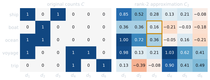
The Frobenius error of $C_2$ is 1.668, and $\sqrt{1.275^2 + 1.000^2 + 0.394^2} = 1.668$, as the layer argument says. The error by rank falls as 2.307, 1.668, 1.075, 0.394, and 0 for $k = 1$ to 5. The spectral norm of $C - C_2$ is 1.275, which is $\sigma_3$, the value in the textbook's statement of the theorem.
To check that no rank-2 matrix does better, two experiments were run. Keeping any other pair of dimensions, for example the first and third, gives a larger error (1.923 for that pair, and up to 2.974 for the fourth and fifth). And minimizing $\|C - AB\|_F$ over all $5 \times 2$ matrices $A$ and $2 \times 6$ matrices $B$ by gradient descent, from 30 random starts, ended at 1.668 every time, never lower.
Step 4: coordinates in two dimensions
Keeping $k = 2$, the documents' coordinates in the reduced space, the columns of $\Sigma_2 V_2^{\mathsf{T}}$, which equal $U_2^{\mathsf{T}} C$, are:
| $d_1$ | $d_2$ | $d_3$ | $d_4$ | $d_5$ | $d_6$ | |
|---|---|---|---|---|---|---|
| Dimension 1 | 1.62 | 0.60 | 0.44 | 0.97 | 0.70 | 0.26 |
| Dimension 2 | −0.46 | −0.84 | −0.30 | 1.00 | 0.35 | 0.65 |
Terms get coordinates the same way, as the rows of $U_2 \Sigma_2$: ship (0.95, −0.47), boat (0.28, −0.53), ocean (1.03, −0.81), voyage (1.52, 0.56), trip (0.57, 1.03).
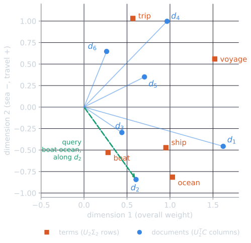
The second dimension separates the sea (negative: ship, boat, ocean) from travel (positive: voyage, trip). Documents $d_2$ (boat ocean) and $d_3$ (ship) share no term, and their cosine in the original space is 0. In the reduced space it is 0.94, because ship, boat, and ocean co-occur and so load on the same dimensions. The same happens to the terms: ship and boat never appear together, and the cosine of their rows of $C$ is 0, but the cosine of their two-dimensional coordinates is 0.81.
The reduction moves every pair of documents, not only the ones with no shared terms:
| Pair | Shared terms | Cosine, original space | Cosine, 2 dimensions |
|---|---|---|---|
| $d_2, d_3$ | none | 0.00 | 0.94 |
| $d_1, d_3$ | ship | 0.58 | 0.95 |
| $d_1, d_2$ | ocean | 0.41 | 0.78 |
| $d_5, d_6$ | none | 0.00 | 0.75 |
| $d_4, d_6$ | trip | 0.71 | 0.93 |
| $d_2, d_6$ | none | 0.00 | −0.53 |
Pairs within one side of the sea/travel divide move closer, whether or not they share a word, and pairs across it move apart, to negative cosines that no pair of count vectors can have. $d_1$, which mixes ship and ocean with voyage, sits between the two groups.
Queries and new documents
A query is a vector $\vec{q}$ in term space, so it must be mapped into the reduced space before it can be compared with documents. The map comes from the decomposition itself. Multiply $C = U \Sigma V^{\mathsf{T}}$ on the left by $U_k^{\mathsf{T}}$. Because the columns of $U$ are orthonormal, $U_k^{\mathsf{T}} U$ is the identity on the first $k$ dimensions and zero on the rest, so $U_k^{\mathsf{T}} C = \Sigma_k V_k^{\mathsf{T}}$, and therefore $V_k^{\mathsf{T}} = \Sigma_k^{-1} U_k^{\mathsf{T}} C$. Each column of $C$, a document in term space, is sent to its column of $V_k^{\mathsf{T}}$ by the matrix $\Sigma_k^{-1} U_k^{\mathsf{T}}$. The same map applies to the query:
$$\vec{q}_k = \Sigma_k^{-1} U_k^{\mathsf{T}} \vec{q}.$$
Documents are then ranked by the cosine between $\vec{q}_k$ and their columns of $V_k^{\mathsf{T}}$.
The query boat ocean
The query vector is $\vec{q} = (0, 1, 1, 0, 0)$ in the term order ship, boat, ocean, voyage, trip. Its projection takes the boat and ocean entries of each column of $U_2$:
$$U_2^{\mathsf{T}} \vec{q} = \begin{pmatrix} 0.129 + 0.476 \\ -0.331 - 0.511 \end{pmatrix} = \begin{pmatrix} 0.605 \\ -0.843 \end{pmatrix}, \qquad \vec{q}_2 = \Sigma_2^{-1} U_2^{\mathsf{T}} \vec{q} = \begin{pmatrix} 0.605 / 2.163 \\ -0.843 / 1.594 \end{pmatrix} = \begin{pmatrix} 0.280 \\ -0.528 \end{pmatrix}.$$
The query happens to contain exactly the words of $d_2$, so it lands on $d_2$'s point. Its cosines with the six documents are:
| $d_1$ | $d_2$ | $d_3$ | $d_4$ | $d_5$ | $d_6$ | |
|---|---|---|---|---|---|---|
| Original space | 0.41 | 1.00 | 0.00 | 0.00 | 0.00 | 0.00 |
| LSI, scaled by $\Sigma_2^{-1}$ | 0.75 | 1.00 | 0.94 | −0.45 | −0.11 | −0.71 |
| LSI, unscaled | 0.78 | 1.00 | 0.94 | −0.18 | 0.16 | −0.53 |
In the original space the query matches only $d_1$ and $d_2$. In the reduced space, $d_3$, which contains only ship, scores 0.94 and ranks second, ahead of $d_1$, which contains ocean itself. That is the synonymy effect LSI was designed for: a document retrieved for a query with which it shares no term.
The table above used the unscaled coordinates $U_k^{\mathsf{T}}\vec{x} = \Sigma_k V_k^{\mathsf{T}}$, while the query formula uses coordinates scaled by $\Sigma_k^{-1}$. In this example the cosine of $d_2$ and $d_3$ is 0.94 either way, but other values differ: with scaling, all three travel documents score below zero; without it, $d_5$ scores slightly above. Whether to scale by $\Sigma_k^{-1}$, by $\Sigma_k$, or not at all is a choice the theory does not settle, and it matters in practice, as the Cranfield experiment below shows. Without scaling, $U_k^{\mathsf{T}}\vec{x}$ is simply the projection of a vector onto the subspace spanned by the first $k$ dimensions, and every dimension keeps the weight it has in the data. Scaling by $\Sigma_k^{-1}$ gives every dimension equal weight, which magnifies the weaker ones.
Folding in documents
A new document can be folded in the same way, mapped into the existing space without recomputing the SVD. A new document boat trip, for instance, gets the unscaled coordinates $U_2^{\mathsf{T}} \vec{x} = (0.129 + 0.263,\ -0.331 + 0.647) = (0.39, 0.32)$, between the sea and travel groups, as a document with one word from each should be. Folding in is cheap, but the dimensions do not change to reflect the new documents, so after many additions the SVD must be recomputed. Terms that are new to the collection are simply dropped, since they have no row in $U$ (Manning, Raghavan, and Schütze, 2008, §18.4).
An experiment on Cranfield
LSI was tested on the Cranfield collection of 1,400 aerodynamics abstracts and 225 queries, with the text processing of comparing ranking models. Documents and queries were weighted by logarithmic term frequency times IDF and normalized to unit length, giving a $4{,}803 \times 1{,}400$ term-document matrix. The baseline is cosine similarity in the full space with the same weights.
| Method | MAP | P@10 |
|---|---|---|
| Cosine, full space | 0.265 | 0.211 |
| LSI, $k = 50$ | 0.321 | 0.247 |
| LSI, $k = 100$ | 0.354 | 0.261 |
| LSI, $k = 200$ | 0.353 | 0.270 |
| LSI, $k = 300$ | 0.334 | 0.257 |
| LSI, $k = 500$ | 0.310 | 0.240 |
| LSI, $k = 800$ | 0.287 | 0.228 |
| BM25, for comparison | 0.307 |
These LSI runs project without scaling. Scaling by $\Sigma_k^{-1}$, as in the textbook's formula, did worse at every $k$, for example 0.327 at $k = 100$ and 0.170 at $k = 800$, probably because it inflates the weakest dimensions, which are the noisiest. The first 100 of the 1,398 dimensions hold 30.8 percent of the squared Frobenius norm, and the first 500 hold 72.5 percent, so even a good reduction discards most of the matrix.
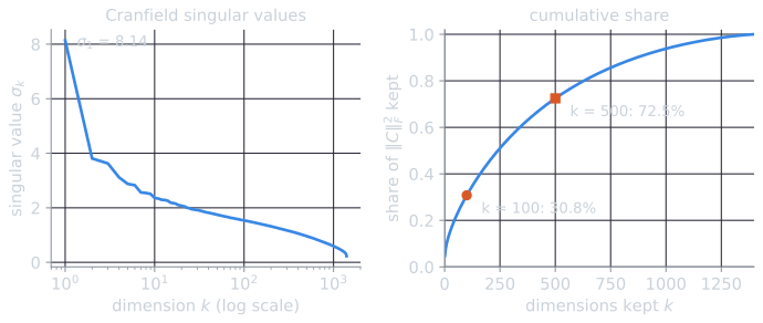
The spectrum explains why the choice of $k$ has to be made empirically. In the five-term example, two dimensions held 72 percent of the matrix. Cranfield's largest singular value, 8.14, stands apart because every column has unit length and positive entries, so the first dimension mostly records the average document. After it, the values fall slowly, from 3.81 for the second to 1.54 for the hundredth and 0.96 for the five-hundredth. Keeping half of the squared norm takes 241 dimensions, and keeping 90 percent takes 868. At $k = 100$ the approximation's error is 83 percent of the norm of $C$ itself. Retrieval improved anyway, which says that what LSI discards is not uniformly noise, but that much of what it keeps is the part that matters for ranking.
Every value of $k$ tested beat the full-space cosine, and every value from 50 to 500 also beat BM25, the strongest model in comparing ranking models, though at $k = 500$ only barely. At $k = 100$, LSI was better than BM25 on 142 of the 225 queries, and a randomization test gave $p < 0.0001$. The best $k$ was chosen on the same queries it is reported on, which slightly overstates it, but the gain does not depend on a single lucky choice. Mixing the full-space and LSI scores did no better than LSI alone.
Where the gain came from
The usual explanation for LSI is that it retrieves relevant documents that share no words with the query, as $d_3$ was retrieved for boat ocean above. On Cranfield, that is not what happened. Only 61 of the 1,612 relevant query-document pairs share no term at all. Of the 2,250 top-ten results LSI returned for the 225 queries, just one shared no term with its query, and it was not relevant. LSI improved the ranking among documents that already matched.
A plausible reading is that the projection changes how much each match counts. In the full space, a match on a rare term that happens to appear in the query carries a large IDF weight even if the document is about something else. In the reduced space, a term counts through the dimensions it loads on, so a match on terms central to the query's subject, and supported by the document's other terms, counts for more than an isolated match. The worked example shows the same effect at small scale: in $C_2$, $d_1$'s weight for ship fell from 1 to 0.85 while $d_3$ gained weight for ocean, because each document's entries were pulled toward the pattern of its dimension. This is a form of smoothing, related in spirit to pseudo-relevance feedback, which also raised MAP on Cranfield, from 0.307 to 0.324, by using the vocabulary of documents that match well.
Cranfield is small and confined to one field, where patterns of co-occurrence are strong and consistent. On larger and more varied collections, results have been more modest. In Dumais's experiments on TREC, LSI achieved precision at or above that of the median participant, its best routing run had the top score on about a fifth of the topics, and it was reported slightly better on average than standard vector space retrieval at about 350 dimensions (Dumais, 1993, 1995; Manning, Raghavan, and Schütze, 2008, §18.4). The textbook also notes cases where it fell short of conventional indexing.
Common misreadings
- "LSI finds synonyms." It finds terms with similar co-occurrence patterns. ship and boat end up close because both appear with ocean, a second-order association: they never appear together. Terms that are true synonyms but appear in different contexts are not brought together, and terms that merely appear in the same contexts, such as voyage and trip in this example or a company's name and its product, are, whether or not they mean the same thing.
- "Each dimension is a topic." Only the first dimension is all of one sign. Every later dimension is a contrast, with positive weights for some terms and negative weights for others, and it is the combination of dimensions, not any one of them, that places a document. Here the second dimension happens to be readable as sea against travel; in a real collection most are not.
- "The approximation removes noise, so a smaller error is better." The rank-$k$ approximation is the best fit to the data, but retrieval is not fitting. On Cranfield, $k = 800$ fits the matrix far better than $k = 100$ and retrieves worse.
Costs and limits
- Computation. The SVD of a large term-document matrix is expensive, and the reduced document vectors are dense, so the efficient sparse inverted index no longer applies. Each query must be compared with every document's $k$-dimensional vector.
- Updates. Folding in new documents degrades the space over time, and recomputing the SVD for a changing collection is costly.
- Interpretation. LSI dimensions are contrasts, with positive and negative entries, not topics. In Reuters, one LSI dimension had dividend announcements at one end and earnings tables at the other. Documents can have negative coordinates, and $C_k$ negative entries, which have no natural meaning.
- Statistical basis. Minimizing squared error implicitly assumes that word counts vary with Gaussian noise, a poor fit for counts that are mostly zero. Probabilistic latent semantic analysis was proposed to put the same idea on a probabilistic footing suited to counts.
The experiments are iir_lsi.py, lsi_walkthrough.py, cranfield_lsi.py, and cranfield_spectrum.py in tools/experiments/topics/ in the site repository, and the figures are drawn by tools/figures/latent-semantic-indexing.py.
References
- Deerwester, S., Dumais, S. T., Furnas, G. W., Landauer, T. K., and Harshman, R. (1990). Indexing by latent semantic analysis. Journal of the American Society for Information Science, 41(6), 391–407.
- Dumais, S. T. (1993). LSI meets TREC: A status report. In Proceedings of the First Text REtrieval Conference (TREC-1), 137–152. NIST Special Publication 500-207.
- Dumais, S. T. (1995). Latent semantic indexing (LSI): TREC-3 report. In Proceedings of the Third Text REtrieval Conference (TREC-3), 219–230. NIST Special Publication 500-225.
- Eckart, C., and Young, G. (1936). The approximation of one matrix by another of lower rank. Psychometrika, 1(3), 211–218.
- Manning, C. D., Raghavan, P., and Schütze, H. (2008). Introduction to Information Retrieval, chapter 18. Cambridge University Press.