The inverted index article built an index by collecting every (term, docID) pair in the collection, sorting them, and grouping the result. For four short documents that is trivial. The Reuters RCV1 collection used throughout Manning, Raghavan, and Schütze's textbook has about 800,000 documents and about 100 million (term, docID) pairs. At four bytes for each term identifier and four for each docID, that is 800 megabytes of pairs to sort, before positions or frequencies are added. A web collection has thousands of times as many. The sorting step that was trivial for four documents becomes the central engineering problem of indexing: how to sort and group far more data than fits in memory.
This article describes the standard algorithms, following Manning, Raghavan, and Schütze (2008, ch. 4). Two build an index on a single machine, one distributes the work across many, and a final group of methods keeps an index up to date as the collection changes.
Why access patterns matter
Index construction is shaped by one fact about storage: reading data sequentially is far faster than reading it at scattered positions. On a spinning disk, moving the read head to a new position takes several milliseconds, during which tens or hundreds of kilobytes could have been read sequentially. Solid-state drives reduce the gap but do not eliminate it, and memory is faster still. An algorithm that sorts 100 million pairs on disk by accessing them in random order would spend nearly all its time seeking.
A rough calculation shows the size of the gap. Assume, for illustration, a disk that needs 5 milliseconds per seek and then transfers 100 megabytes per second. Reading RCV1's 800 megabytes of pairs sequentially takes $800 / 100 = 8$ seconds. Fetching the same 100 million pairs one at a time from random positions takes $10^{8} \times 5\ \text{ms} = 5 \times 10^{5}$ seconds, nearly six days. The exact figures vary from device to device, but the ratio of several orders of magnitude is the reason every algorithm below is organized around long sequential reads and writes. Efficient construction algorithms therefore do as much work as possible in memory, write data to disk in large sequential blocks, and read it back sequentially.
Blocked sort-based indexing
Blocked sort-based indexing (BSBI) applies the textbook method one memory-sized block at a time (Manning, Raghavan, and Schütze, 2008, §4.2):
- Divide the collection into blocks small enough that each block's pairs fit in memory.
- For each block:
- parse the documents into (termID, docID) pairs, using a dictionary that maps each term to an integer termID;
- sort the pairs in memory;
- group them into postings lists for that block, and write the block's partial index to disk.
- Merge the block indexes into the final index.
The merge reads all block files simultaneously, a small buffer from each, and repeatedly takes the smallest termID among the buffers. Postings for the same term from different blocks are concatenated, which keeps them in docID order, because the blocks cover increasing ranges of docIDs. A priority queue finds the smallest termID efficiently. Every block file is read once, sequentially, and the final index is written once, sequentially.
For RCV1, Manning, Raghavan, and Schütze describe ten blocks of about ten million pairs each. The cost is dominated by sorting, so the total running time grows as $\Theta(T \log T)$ for $T$ pairs.
BSBI on a small example
The four documents of the inverted index article make the steps concrete. After lowercasing, removing in, and Porter stemming, they are:
| docID | Terms |
|---|---|
| 1 | new home sale top forecast |
| 2 | home sale rise juli |
| 3 | increas home sale juli |
| 4 | juli new home sale rise |
Suppose memory holds only about nine pairs, so the collection is processed in two blocks of two documents. BSBI first needs termIDs. Assigning them in order of first appearance gives new = 1, home = 2, sale = 3, top = 4, forecast = 5, rise = 6, juli = 7, increas = 8. This map is global: when block 2 meets home, it must use the same number, 2, that block 1 used.
| Block | Pairs (termID, docID) as parsed | After sorting |
|---|---|---|
| 1 (docs 1, 2) | (1,1) (2,1) (3,1) (4,1) (5,1) (2,2) (3,2) (6,2) (7,2) | (1,1) (2,1) (2,2) (3,1) (3,2) (4,1) (5,1) (6,2) (7,2) |
| 2 (docs 3, 4) | (8,3) (2,3) (3,3) (7,3) (7,4) (1,4) (2,4) (3,4) (6,4) | (1,4) (2,3) (2,4) (3,3) (3,4) (6,4) (7,3) (7,4) (8,3) |
Grouping each sorted block gives its partial index, which is written to disk:
- Block 1: 1 → 1; 2 → 1, 2; 3 → 1, 2; 4 → 1; 5 → 1; 6 → 2; 7 → 2.
- Block 2: 1 → 4; 2 → 3, 4; 3 → 3, 4; 6 → 4; 7 → 3, 4; 8 → 3.
The merge keeps a priority queue holding the next termID from each block. It pops the smallest, appends that block's postings for the term to the output, and pushes the block's following termID. The first pops are termID 1 from block 1, giving the list (1), then termID 1 from block 2, extending it to (1, 4). TermID 2 follows the same way, ending as (1, 2, 3, 4). TermIDs 4 and 5 occur only in block 1 and are copied straight through. Thirteen pops produce the final index, one per (term, block) entry:
| termID | Term | Postings |
|---|---|---|
| 1 | new | 1, 4 |
| 2 | home | 1, 2, 3, 4 |
| 3 | sale | 1, 2, 3, 4 |
| 4 | top | 1 |
| 5 | forecast | 1 |
| 6 | rise | 2, 4 |
| 7 | juli | 2, 3, 4 |
| 8 | increas | 3 |
The postings are the same as those of the in-memory sort, but the lists come out in termID order, not alphabetical order. A dictionary sorted by term, needed for prefix search, is a separate step. Every posting of block 1 has a smaller docID than every posting of block 2, so appending block 2's postings after block 1's keeps every list sorted without comparing docIDs.
At a larger scale, the same procedure applied to Reuters-21578 (Lewis, 1997), a collection of 10,788 news stories tokenized as in the term statistics article, with its 725,793 distinct (term, document) pairs, in blocks of 100,000 pairs produces eight block files and an eight-way merge, in which each pop from the priority queue costs about $\log_2 8 = 3$ comparisons.
BSBI has a weakness: it needs the mapping from terms to termIDs for the whole collection, kept in memory throughout the build. For a very large collection that dictionary may itself be too large, and, as Heaps' law predicts, it keeps growing as long as new documents arrive.
Single-pass in-memory indexing
Single-pass in-memory indexing (SPIMI), described by Heinz and Zobel (2003), avoids both the global dictionary and the sort of pairs:
- Process the documents as a stream. For each token, look up its term in a dictionary for the current block only. If the term is new to the block, create an empty postings list for it. Append the docID to the term's postings list, unless the list already ends with that docID, in which case only the posting's term frequency, if one is stored, is incremented.
- When memory is full, sort the block's terms (not its pairs), write the block's dictionary and postings to disk in term order, and start a new block with an empty dictionary.
- Merge the blocks as in BSBI.
Because each block has its own dictionary of actual terms, no global termID mapping is needed, and blocks can be arbitrarily large given enough memory. Because postings are appended directly to the list for their term, the pairs never need sorting. Only each block's distinct terms are sorted, and there are far fewer of those. Documents are processed in docID order, so each list is already sorted by docID. Building the blocks therefore takes time linear in the collection size, $\Theta(T)$, though the final merge of the blocks adds its own cost. Postings can also be compressed as blocks are written, which reduces the disk traffic of the merge.
SPIMI on the same example
With the same two blocks, SPIMI never assigns termIDs. Block 1 starts with an empty dictionary and reads document 1: new, home, sale, top, and forecast are all new to the block, so each gets a list containing 1. Document 2 then appends 2 to the existing lists of home and sale and creates new lists for rise and juli. When memory is full, the block's seven terms, not its nine postings, are sorted, and the block is written in term order:
| Block 1 (docs 1, 2) | Block 2 (docs 3, 4) |
|---|---|
| forecast → 1 | home → 3, 4 |
| home → 1, 2 | increas → 3 |
| juli → 2 | juli → 3, 4 |
| new → 1 | new → 4 |
| rise → 2 | rise → 4 |
| sale → 1, 2 | sale → 3, 4 |
| top → 1 |
Block 2 builds a fresh dictionary that knows nothing of block 1. All six of its terms are new to it, including home, sale, juli, new, and rise, which block 1 has already seen. Only increas is new to the collection. The merge then works exactly as in BSBI, comparing terms instead of termIDs, and produces the same postings, this time already in alphabetical order. The only sort was of the terms of each block.
The price of forgetting the vocabulary between blocks is that a term occurring in several blocks has a dictionary entry in each. Measured on Reuters-21578 in blocks of about 100,000 postings:
| Block | Postings | Terms in this block (SPIMI) | Terms seen so far (BSBI's map) |
|---|---|---|---|
| 1 | 100,129 | 10,851 | 10,851 |
| 2 | 100,002 | 10,564 | 15,252 |
| 3 | 100,061 | 10,972 | 18,815 |
| 4 | 100,223 | 10,623 | 21,529 |
| 5 | 100,113 | 10,793 | 24,046 |
| 6 | 100,052 | 10,762 | 26,228 |
| 7 | 100,045 | 11,342 | 28,548 |
| 8 | 25,168 | 5,080 | 29,187 |
Each SPIMI block holds a dictionary of about 11,000 terms, roughly constant from block to block, while the map BSBI must keep in memory grows with the collection, as Heaps' law predicts, to 29,187 terms. Summed over the blocks, SPIMI writes 80,987 dictionary entries, 2.77 times the number of distinct terms, and the merge combines them. For this small collection either approach fits easily in memory. The difference matters when the global vocabulary runs to hundreds of millions of terms while each block's stays bounded by the block size.
The algorithm is simple enough that most straightforward indexers, including the indexers built on a dictionary of lists or sets in course projects, are essentially SPIMI without the block flushing. They work until the collection outgrows memory. The pipeline article discusses this in the context of my own homework.
Distributed indexing
When a collection is too large for one machine to index in reasonable time, construction is distributed. Manning, Raghavan, and Schütze (2008, §4.4) describe indexing with MapReduce (Dean and Ghemawat, 2004), a framework that runs a computation in two phases across a cluster:
- In the map phase, many parsers each process a portion of the collection, called a split. Each parser emits (term, docID) pairs and writes them to local files called segments, partitioned by term range. For example, with three partitions, terms beginning a to f go to one segment, g to p to a second, and q to z to a third.
- In the reduce phase, each inverter is assigned one term range. It collects that range's segment files from every parser, sorts the pairs, and writes the postings for its terms.
On the four-document example, with two parsers (documents 1 and 2, and documents 3 and 4) and the three term ranges above:
| Segment a–f | Segment g–p | Segment q–z | |
|---|---|---|---|
| Parser 1 | (forecast,1) | (new,1) (home,1) (home,2) (juli,2) | (sale,1) (top,1) (sale,2) (rise,2) |
| Parser 2 | none | (increas,3) (home,3) (juli,3) (juli,4) (new,4) (home,4) | (sale,3) (sale,4) (rise,4) |
| Inverter output | forecast → 1 | home → 1, 2, 3, 4; increas → 3; juli → 2, 3, 4; new → 1, 4 | rise → 2, 4; sale → 1, 2, 3, 4; top → 1 |
Each inverter reads one column, from every parser, and sorts only that column's pairs. The columns are uneven, ten pairs in the middle range against one in the first. Ranges split by first letter are rarely balanced, because letters begin very different numbers of words and terms differ enormously in frequency. Ranges chosen so that the partitions carry similar amounts of work are better, since the job finishes only when the slowest inverter does.
The framework handles scheduling, moves data between machines, and restarts tasks that fail. Partitioning by term range produces an index divided by term. As described in search at scale, large search engines usually serve indexes divided by document instead. The same framework can produce document-partitioned indexes by partitioning on docID, or a term-partitioned index can be reorganized after construction.
Keeping the index current
Collections change. Documents are added, deleted, and modified, and an index built once and never updated soon becomes stale. Rebuilding from scratch is simple but slow, and a news or web index cannot wait. Manning, Raghavan, and Schütze (2008, §4.5) describe several schemes.
Auxiliary index. Keep the large main index on disk and a small auxiliary index in memory. New documents are indexed into the auxiliary index. Queries are run against both, and their results are combined. Deleted documents are recorded in an invalidation bit vector, one bit per docID, and filtered out of results. A modified document is treated as a deletion followed by an addition. When the auxiliary index fills memory, it is merged into the main index.
The cost of that merge is the problem. Each merge rewrites the entire main index, which keeps growing. If the auxiliary index holds $n$ postings and the collection eventually reaches $T$ postings, there are about $T/n$ merges, each touching up to $T$ postings, so the total work grows as $\Theta(T^2/n)$. For a large and growing collection that is too slow.
Logarithmic merging. Instead of a single main index, keep a series of indexes of sizes $n$, $2n$, $4n$, $8n$, and so on, with at most one of each size. When the in-memory index fills, write it to disk as an index of size $n$. If an index of that size already exists, merge the two into one of size $2n$. If one of size $2n$ already exists, merge again into one of size $4n$, and so on, like carrying digits when adding 1 in binary. Each posting is merged at most about $\log_2(T/n)$ times, so the total work falls to $\Theta(T \log(T/n))$. The price is that a query must consult up to $\log_2(T/n)$ indexes instead of two. Lester, Moffat, and Zobel (2005) analyzed a family of such geometric partitioning schemes, which let a system trade update cost against query cost.
The first few flushes show the binary-counter behaviour. Write $I_0, I_1, I_2, \dots$ for on-disk indexes of sizes $n, 2n, 4n, \dots$:
| Flush | Before | Merges | After | Postings written | Indexes on disk |
|---|---|---|---|---|---|
| 1 | none | none | $I_0$ | $n$ | 1 |
| 2 | $I_0$ | memory + $I_0$ | $I_1$ | $2n$ | 1 |
| 3 | $I_1$ | none | $I_0, I_1$ | $n$ | 2 |
| 4 | $I_0, I_1$ | memory + $I_0$, then + $I_1$ | $I_2$ | $2n + 4n = 6n$ | 1 |
| 5 | $I_2$ | none | $I_0, I_2$ | $n$ | 2 |
| 6 | $I_0, I_2$ | memory + $I_0$ | $I_1, I_2$ | $2n$ | 2 |
| 7 | $I_1, I_2$ | none | $I_0, I_1, I_2$ | $n$ | 3 |
| 8 | $I_0, I_1, I_2$ | three carries | $I_3$ | $2n + 4n + 8n = 14n$ | 1 |
The set of indexes present after flush $j$ matches the binary digits of $j$: after flush 6, binary 110, there are indexes of sizes $2n$ and $4n$. The total written after eight flushes is $28n$. The auxiliary scheme, rewriting the whole main index at each flush, writes $n + 2n + \dots + 8n = 36n$ over the same eight flushes. The gap is small at first and widens quickly: the auxiliary scheme's total grows with the square of the number of flushes, the logarithmic one only slightly faster than linearly.
Simulating both on Reuters-21578 makes the difference concrete. The stories are added in order, each contributing one posting per distinct term, with an in-memory index of $n = 10{,}000$ postings, so the 725,793 postings cause 72 flushes:
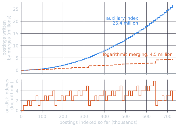
Both totals agree with the analysis. The auxiliary scheme writes about $P^2 / 2n$ postings for a final index of $P$ postings, here $725{,}793^2 / 20{,}000 \approx 26.3$ million. Logarithmic merging writes each posting about once per level it passes through, roughly $P \log_2(P/n) \approx 4.5$ million in total (here 4.47 million). Raising $n$ to 50,000 reduces the auxiliary scheme to 5.3 million postings written and the logarithmic one to 2.1 million: more memory helps both, but it does not change the quadratic shape. In both simulations a merge's cost is counted as the number of postings it writes, including every intermediate result, as in the table above.
This is how widely used systems work. Lucene writes new documents into small immutable segments, searches all current segments together, marks deleted documents in a per-segment bitmap, and merges segments in the background according to a policy that groups segments of similar size. That is logarithmic merging with refinements. Because a segment's postings are never modified once written, readers can search a fixed snapshot of the segments without locks while new segments are being written, and reopen the index to see newer ones.
Deletions and statistics. Deleted documents still occupy space, and their postings still count toward term statistics, until a merge physically removes them. Collection statistics such as document frequency and average document length are therefore approximate between merges. When deletions are few, the error is small, but a collection with heavy deletion should be merged regularly so that its statistics stay accurate.
Summary
| Method | Main idea | Running time | Needs in memory |
|---|---|---|---|
| In-memory sort | Sort all (term, docID) pairs at once | $\Theta(T \log T)$ | All pairs |
| BSBI | Sort pairs block by block, then merge | $\Theta(T \log T)$ | One block of pairs and the global term-to-termID map |
| SPIMI | Append postings to per-block term lists, then merge | $\Theta(T)$ before the merge | One block's dictionary and postings |
| MapReduce | Parse in parallel, partition by term, invert in parallel | Divided across machines | One split per parser, one partition per inverter |
| Logarithmic merging | Keep indexes of doubling sizes and merge like binary carries | $\Theta(T \log(T/n))$ for updates | The current in-memory index |
The algorithms differ in how they use memory and disk, but they share one goal: the index is built and maintained by sequential passes over large blocks of data. The next article, index compression, reduces the size of those blocks, which cuts the disk traffic of every one of these algorithms at the cost of some decoding work.
References
- Dean, J., and Ghemawat, S. (2004). MapReduce: Simplified data processing on large clusters. In Proceedings of OSDI 2004, 137–150.
- Heinz, S., and Zobel, J. (2003). Efficient single-pass index construction for text databases. Journal of the American Society for Information Science and Technology, 54(8), 713–729.
- Lester, N., Moffat, A., and Zobel, J. (2005). Fast on-line index construction by geometric partitioning. In Proceedings of CIKM 2005, 776–783.
- Lewis, D. D. (1997). Reuters-21578 text categorization test collection, distribution 1.0.
- Manning, C. D., Raghavan, P., and Schütze, H. (2008). Introduction to Information Retrieval, chapter 4. Cambridge University Press.