The postings of the Reuters RCV1 collection contain about 100 million document identifiers. Stored as 32-bit integers, they occupy 400 megabytes. Encoded with the two simple codes described in this article, the same postings occupy about 116 megabytes with variable byte codes and about 101 megabytes with Elias gamma codes, roughly a quarter of the original size (Manning, Raghavan, and Schütze, 2008, §5.3). The dictionary can be reduced from 11.2 megabytes to about 5.9. None of this loses any information.
Compression matters for speed as well as space. A compressed index lets more of the postings stay in memory, and the parts that must be read from disk transfer faster. Decompressing simple codes is quick, so reading compressed postings and decoding them is usually faster than reading uncompressed postings. This article covers the classic methods for the dictionary and the postings, following Manning, Raghavan, and Schütze (2008, ch. 5), and then the codes used in current systems.
Lossless and lossy
The compression in this article is lossless: the original index can be reconstructed exactly. Several earlier steps in text processing are, in effect, lossy compression. Stop-word removal, case folding, and stemming each discard distinctions to make the index smaller, and the discarded information cannot be recovered. Static index pruning goes further, removing postings that are unlikely to affect the top results of any query (Carmel et al., 2001). Lossy methods change what the index can answer. Lossless methods only change how it is stored.
Compressing the dictionary
The dictionary is small compared with the postings, but it should stay in memory, since every query consults it. The RCV1 dictionary has about 400,000 terms.
Fixed-width entries. The simplest layout is an array of fixed-size entries, each with 20 bytes for the term, 4 bytes for its document frequency, and 4 bytes for a pointer to its postings list. At 28 bytes per entry, the dictionary needs $400{,}000 \times 28 = 11.2$ megabytes. Most of that is wasted, because the average English term is about 8 characters long, while the 20-byte field must fit the longest terms, and still cannot fit some.
Dictionary as a string. Store all the terms, sorted, in one long string, and give each array entry a pointer into that string instead of the term itself. A pointer to one of about 3.2 million character positions needs 3 bytes. Each entry now needs 4 bytes for frequency, 4 for the postings pointer, 3 for the term pointer, and an average of 8 characters in the string, a total of 19 bytes, or $400{,}000 \times 19 = 7.6$ megabytes.
Blocking. Group the terms into blocks of $k$ and keep a string pointer only for the first term of each block, storing each term's length as a single byte before it in the string. With $k = 4$, each block saves three 3-byte pointers (9 bytes) and adds four 1-byte lengths (4 bytes), a net saving of 5 bytes per four terms. That removes $400{,}000 / 4 \times 5 = 500{,}000$ bytes, bringing the dictionary to 7.1 megabytes. The cost is lookup speed: binary search finds the right block, and then the terms within the block are scanned in sequence.
Front coding. Sorted terms share prefixes with their neighbors, so within a block the shared prefix can be written once. The four terms automata, automate, automatic, and automation are stored with blocking as
8automata8automate9automatic10automation
which is 40 characters. With front coding, the common prefix automat is written once, followed by each term's remaining characters:
8automat*a1◊e2◊ic3◊ion
Here 8automat*a gives the first term, of length 8, with * marking the end of the shared prefix automat. Each later term is then given by the number of extra characters, a ◊, and those characters: 1◊e is automate, 2◊ic is automatic, and 3◊ion is automation. The block shrinks from 40 characters to 22. Front coding brings the RCV1 dictionary to about 5.9 megabytes (Manning, Raghavan, and Schütze, 2008, §5.2).
The same steps on a real dictionary
The same calculations can be run on a dictionary small enough to inspect. Reuters-21578 (Lewis, 1997), a collection of 10,788 news stories, has 29,187 distinct terms when its text is lowercased and split into runs of letters, as in the term statistics article. Their average length is 6.99 characters, and together they take 203,992 characters. A pointer into a string of that length needs $\lceil \log_2 203{,}992 \rceil = 18$ bits, so 3 bytes, as for RCV1. Each layout's size is the sum of its parts:
| Layout | Bytes per term (or block) | Total |
|---|---|---|
| Fixed width | 20 + 4 + 4 = 28 | 817.2 kB |
| Dictionary as a string | 4 + 4 + 3 + 6.99 = 17.99 | 525.0 kB |
| Blocking, $k = 4$ | 4 + 4 + 1 length byte + 6.99, plus 3 per block | 488.6 kB |
| Blocking and front coding, $k = 4$ | as above, minus each block's repeated prefixes | 422.5 kB |
(Kilobytes are thousands of bytes, rounded to one decimal.) The fixed-width layout fails in the other direction too: four of the terms are longer than 20 characters and would not fit. The front-coded size counts, for each block, one byte for the length of the shared prefix, the first term in full with its length byte, and each later term as a length byte plus the characters after the shared prefix. A real block shows where the savings come from. The four consecutive terms computer, computerised, computerization, and computerized share the prefix computer. Blocked, they take $9 + 13 + 16 + 13 = 51$ bytes. Front coded, in the textbook's notation,
8computer*4◊ised7◊ization4◊ized
they take 28 bytes: 1 for the prefix length, 9 for the first term, and $5 + 8 + 5$ for the other three. Larger blocks save more pointer bytes but make lookups scan further. On this dictionary, blocks of 8 bring the front-coded size to 412.1 kB, and blocks of 16 to 412.3 kB, slightly larger, because the common prefix of sixteen consecutive terms is usually shorter than that of four.
Compressing the postings: gaps
A postings list is a sorted sequence of docIDs, and docIDs in a large collection are large numbers. The key observation is that a sorted list can be stored as the differences between consecutive entries, called gaps or d-gaps, from which the original list is recovered by adding them up. Manning, Raghavan, and Schütze (2008, §5.3) give three lists:
| Term | docIDs | Gaps |
|---|---|---|
| the | 283042, 283043, 283044, 283045 | 283042, 1, 1, 1 |
| computer | 283047, 283154, 283159, 283202 | 283047, 107, 5, 43 |
| arachnocentric | 252000, 500100 | 252000, 248100 |
Frequent terms, which have the longest lists, have the smallest gaps, often 1. Rare terms have large gaps, but their lists are short. This is the distribution described by Zipf's law, and it is what makes postings compressible: most of the numbers stored in an index are small. A variable-length code, which uses few bits for small numbers and more bits for large ones, exploits it.
Two real lists from Reuters-21578, with the stories numbered 1 to 10,788 in order of their Reuters identifiers, which is roughly the order they were filed, carry through the rest of this article. Palladium, a rare term, occurs in five stories. Oil occurs in 1,038, and its first ten postings are shown:
| Term | docIDs | Gaps |
|---|---|---|
| palladium | 1467, 1521, 1792, 1795, 8079 | 1467, 54, 271, 3, 6284 |
| oil (first ten) | 3, 39, 80, 91, 94, 95, 101, 119, 121, 126 | 3, 36, 41, 11, 3, 1, 6, 18, 2, 5 |
The gaps of palladium are mostly large, since five postings are spread over ten thousand stories, though two of them, 3 and 54, are small. The gaps of oil are small, with an average of 10.4 over the whole list (rounded to one decimal), because a story mentioning oil appears every few stories. Across the whole collection, 15 percent of all gaps are exactly 1, 80 percent are below 128, and none can reach 16,384, since there are only 10,788 stories.
Variable byte codes
Variable byte (VB) encoding uses a whole number of bytes for each gap. The low 7 bits of each byte carry data, and the high bit, the continuation bit, marks the last byte of a number. In the convention of Manning, Raghavan, and Schütze, it is set to 1 on the last byte and 0 on the others. Many implementations use the opposite convention, setting the bit to 1 when more bytes follow. Either works, as long as the encoder and decoder agree. To encode a gap, split its binary representation into 7-bit groups:
| Gap | VB encoding |
|---|---|
| 1 | 10000001 |
| 5 | 10000101 |
| 130 | 00000001 10000010 |
| 824 | 00000110 10111000 |
| 214577 | 00001101 00001100 10110001 |
For 824, the binary representation is 110 0111000, which splits into the 7-bit groups 0000110 and 0111000. The first byte carries 0000110 with continuation bit 0, and the last carries 0111000 with continuation bit 1. A decoder reads bytes, accumulating 7 bits at a time, until it reads a byte whose high bit is 1. Gaps below 128 take one byte, and gaps below 16,384 take two.
VB codes are simple and fast to decode, because they work on whole bytes, and they reduce RCV1's postings from 400 to about 116 megabytes.
Variable byte on a real list
Encoding the gaps of palladium one at a time:
| Gap | Binary | 7-bit groups | VB bytes |
|---|---|---|---|
| 1467 | 10110111011 |
0001011 0111011 |
00001011 10111011 |
| 54 | 110110 |
0110110 |
10110110 |
| 271 | 100001111 |
0000010 0001111 |
00000010 10001111 |
| 3 | 11 |
0000011 |
10000011 |
| 6284 | 1100010001100 |
0110001 0001100 |
00110001 10001100 |
The 7-bit groups are taken from the right, so the leftmost group is padded with zeros. Each group then receives its continuation bit: 0 on every byte but the last of a number, 1 on the last. The five gaps take 8 bytes, 64 bits, against 160 bits as 32-bit integers. The stored stream is
00001011 10111011 10110110 00000010 10001111 10000011 00110001 10001100
Decoding needs no separators. Start with $n = 0$. The first byte, 00001011, has high bit 0, so it is not the last: $n = 128 \times 0 + 11 = 11$. The second, 10111011, has high bit 1, so it ends the number: its low 7 bits are 59, and $n = 128 \times 11 + 59 = 1467$. Reset $n$ to 0 and continue: 10110110 ends at once, giving 54, and so on. Adding the gaps back up, $1467$, $1467 + 54 = 1521$, $1521 + 271 = 1792$, and so on, recovers the docIDs.
For the first ten postings of oil, every gap is below 128, so each takes exactly one byte, 80 bits in all. One byte per gap is also the floor for VB: a gap of 1 costs as much as a gap of 127.
Elias gamma codes
Byte alignment wastes space on small gaps: a gap of 1, the most common value in many lists, still takes eight bits. Bit-level codes can do better. The Elias gamma code (Elias, 1975) represents a positive integer $G$ in two parts:
- the offset: $G$ in binary with the leading 1 removed, since every positive integer's binary form begins with 1;
- the length: the number of bits in the offset, written in unary, as that many 1s followed by a 0.
The code is the length followed by the offset. For 13, binary 1101, the offset is 101, three bits long, so the length is 1110, and the code is 1110101:
| Gap | Length | Offset | Gamma code | Bits |
|---|---|---|---|---|
| 1 | 0 |
0 |
1 | |
| 2 | 10 |
0 |
100 |
3 |
| 5 | 110 |
01 |
11001 |
5 |
| 9 | 1110 |
001 |
1110001 |
7 |
| 13 | 1110 |
101 |
1110101 |
7 |
| 24 | 11110 |
1000 |
111101000 |
9 |
| 511 | 111111110 |
11111111 |
11111111011111111 |
17 |
| 1025 | 11111111110 |
0000000001 |
111111111100000000001 |
21 |
A gamma code for $G$ takes $2\lfloor \log_2 G \rfloor + 1$ bits, about twice the minimum needed to write $G$ in binary. The count follows from the construction. $G$ has $\lfloor \log_2 G \rfloor + 1$ binary digits, so its offset has $\lfloor \log_2 G \rfloor$. The unary length spends one 1 for each offset bit plus a closing 0. Adding the two parts gives $2\lfloor \log_2 G \rfloor + 1$. For 13, $\lfloor \log_2 13 \rfloor = 3$, and the code has $2 \times 3 + 1 = 7$ bits. The code is prefix-free, meaning no code is the beginning of another, so a sequence of codes can be decoded without separators: read 1s until a 0 to learn the length, then read that many bits of offset. It is also parameter-free, so it needs no tuning to a particular collection. Gamma codes reduce RCV1's postings to about 101 megabytes, smaller than VB.
Gamma on the same lists
For the rare term palladium:
| Gap | Length (unary) | Offset | Bits |
|---|---|---|---|
| 1467 | 11111111110 |
0110111011 |
21 |
| 54 | 111110 |
10110 |
11 |
| 271 | 111111110 |
00001111 |
17 |
| 3 | 10 |
1 |
3 |
| 6284 | 1111111111110 |
100010001100 |
25 |
The list takes 77 bits, more than the 64 of variable byte. Large gaps are where gamma is weak: its unary length grows one bit for every doubling of the gap, so it spends about $2\log_2 G$ bits where VB spends about $\frac{8}{7}\log_2 G$, rounded up to whole bytes. For the first ten postings of oil the comparison reverses:
| Gap | Gamma code | Bits | VB bits |
|---|---|---|---|
| 3 | 101 |
3 | 8 |
| 36 | 11111000100 |
11 | 8 |
| 41 | 11111001001 |
11 | 8 |
| 11 | 1110011 |
7 | 8 |
| 3 | 101 |
3 | 8 |
| 1 | 0 |
1 | 8 |
| 6 | 11010 |
5 | 8 |
| 18 | 111100010 |
9 | 8 |
| 2 | 100 |
3 | 8 |
| 5 | 11001 |
5 | 8 |
Gamma needs 58 bits for these ten gaps, against 80 for VB. Over the whole list of 1,038 postings it needs 5,728 bits, 5.5 bits per posting, against VB's 8. Decoding the stream 1011111000100... shows that the codes need no separators: read 1s up to the first 0 (one 1, so the offset has one bit), read one bit (1), and restore the leading 1 to get binary 11, which is 3. Then 111110 announces a five-bit offset, 00100, giving binary 100100, which is 36.
Codes that encode the length itself more efficiently, such as Elias delta codes, do better for large gaps. A delta code writes the number of binary digits of $G$ as a gamma code, followed by the same offset. For 1467, which has 11 binary digits, that is the gamma code of 11, 1110011, followed by the 10-bit offset 0110111011, 17 bits instead of gamma's 21. For small gaps delta can be slightly longer: 2 takes 3 bits in gamma and 4 in delta. Golomb and Rice codes, which take a parameter fitted to each list, do better still when gaps follow a geometric distribution (Witten, Moffat, and Bell, 1999).
Measured on a whole collection
Applying each code to every postings list of Reuters-21578, 725,793 postings in all, gives the following sizes (megabytes of a million bytes, rounded to three decimals; bits per posting rounded to two):
| Encoding of the docIDs | Size | Bits per posting |
|---|---|---|
| 32-bit integers | 2.903 MB | 32.00 |
| Fixed 14-bit integers, the fewest that can hold 10,788 | 1.270 MB | 14.00 |
| VB on the docIDs themselves, no gaps | 1.445 MB | 15.93 |
| VB on gaps | 0.868 MB | 9.57 |
| Gamma on gaps | 0.783 MB | 8.63 |
| Delta on gaps | 0.733 MB | 8.08 |
| zlib (level 9) on the 32-bit gaps | 0.909 MB | 10.02 |
Several lessons are in the table. Gaps matter more than the choice of code: VB on raw docIDs saves half, VB on gaps saves 70 percent. Even the simplest gap code beats a fixed-width encoding sized exactly to the collection. And a general-purpose compressor, zlib, which knows nothing of the structure of postings, does worse than either of the integer codes, despite working much harder.
The averages hide a strong dependence on the term. Grouping terms by document frequency:
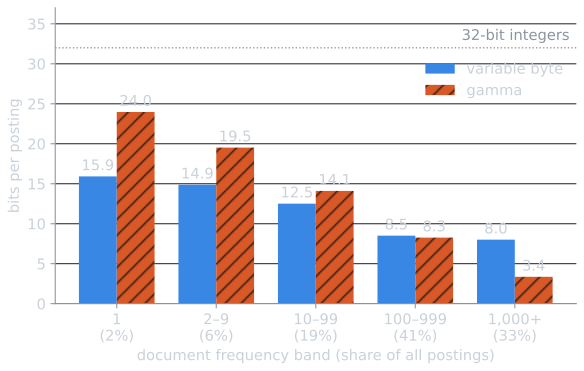
The crossover is at document frequencies of about a hundred: below it variable byte is smaller, and from the 100 to 999 band upward gamma is. Rare terms, which make up most of the dictionary, cost gamma more. Frequent terms, which hold most of the postings, cost it much less. Since the size of an index is dominated by its long lists, the code that is better on long lists wins, which is the Zipf's law skew at work.
Size against speed
Bit-level codes produce smaller indexes, but decoding them means extracting individual bits, which processors do slowly. Scholer, Williams, Yiannis, and Zobel (2002) found that byte-aligned codes gave faster query processing than bit-aligned ones despite being larger, because decoding speed mattered more than the size difference. Later work has pushed further in the same direction, toward codes designed for how processors actually work:
- Word-aligned codes such as Simple-9 pack as many small gaps as fit into each 32-bit word, using a few bits of the word to say how they are packed (Anh and Moffat, 2005).
- PForDelta encodes blocks of, typically, 128 gaps with a fixed bit width chosen to fit most of them, and stores the few large exceptions separately, so that most values can be decoded with no branching (Zukowski, Héman, Nes, and Boncz, 2006).
- SIMD codecs decode several integers at once using the vector instructions of modern processors, reaching billions of integers per second (Lemire and Boytsov, 2015).
Pibiri and Venturini (2021) survey these and other methods. Production search engines typically use block-based codes of this kind, often combined with skip information that lets a query jump over blocks it does not need, which connects compression to the skip pointers used in postings intersection.
Making gaps smaller
Gaps depend on how docIDs are assigned. If documents that share many terms receive nearby docIDs, the postings lists of those terms contain runs of small gaps, which compress better. DocID reassignment reorders the collection before indexing, for example by clustering similar documents or, on the web, sorting pages by URL so that pages from the same site are adjacent (Silvestri, 2007). Reassignment can substantially reduce index size without changing any code.
Reuters-21578 shows the effect in a mild form. Its stories are numbered roughly in filing order, so stories about the same event tend to be near each other. Shuffling the docIDs into a random order, with 30 different random seeds, raises the gamma-coded size from 0.783 to a median of 0.815 megabytes (interquartile range 0.815 to 0.816), about 4 percent, and the VB size from 0.868 to a median of 0.876 megabytes. Filing order is a weak form of clustering. Orderings designed to put similar documents together, such as the URL sorting described above, are what produce the large savings.
The same gap technique applies to the positions in a positional index: positions within a document are stored as gaps between successive occurrences, and term frequencies, which are mostly small numbers, are encoded with the same variable-length codes.
Summary
| Structure | Method | RCV1 size |
|---|---|---|
| Dictionary | Fixed-width entries | 11.2 MB |
| Dictionary as a string | 7.6 MB | |
| String with blocking, $k = 4$ | 7.1 MB | |
| Blocking and front coding | 5.9 MB | |
| Postings (docIDs) | 32-bit integers | 400 MB |
| Variable byte codes on gaps | 116 MB | |
| Elias gamma codes on gaps | 101 MB |
The first three dictionary sizes and the uncompressed postings size are computed in this article. The front-coding and compressed postings sizes are those reported by Manning, Raghavan, and Schütze (2008, §§5.2–5.3).
Compression is what makes many other design decisions affordable. It is one reason web engines can keep stop words in the index, since their long lists of small gaps compress to very little, and it lets a large share of a production index be served from memory, as described in search at scale.
References
- Anh, V. N., and Moffat, A. (2005). Inverted index compressed using word-aligned binary codes. Information Retrieval, 8(1), 151–166.
- Carmel, D., Cohen, D., Fagin, R., Farchi, E., Herscovici, M., Maarek, Y. S., and Soffer, A. (2001). Static index pruning for information retrieval systems. In Proceedings of SIGIR 2001, 43–50.
- Elias, P. (1975). Universal codeword sets and representations of the integers. IEEE Transactions on Information Theory, 21(2), 194–203.
- Lemire, D., and Boytsov, L. (2015). Decoding billions of integers per second through vectorization. Software: Practice and Experience, 45(1), 1–29.
- Lewis, D. D. (1997). Reuters-21578 text categorization test collection, distribution 1.0.
- Manning, C. D., Raghavan, P., and Schütze, H. (2008). Introduction to Information Retrieval, chapter 5. Cambridge University Press.
- Pibiri, G. E., and Venturini, R. (2021). Techniques for inverted index compression. ACM Computing Surveys, 53(6), article 125.
- Scholer, F., Williams, H. E., Yiannis, J., and Zobel, J. (2002). Compression of inverted indexes for fast query evaluation. In Proceedings of SIGIR 2002, 222–229.
- Silvestri, F. (2007). Sorting out the document identifier assignment problem. In Proceedings of ECIR 2007, 101–112.
- Witten, I. H., Moffat, A., and Bell, T. C. (1999). Managing Gigabytes: Compressing and Indexing Documents and Images, 2nd edition. Morgan Kaufmann.
- Zukowski, M., Héman, S., Nes, N., and Boncz, P. (2006). Super-scalar RAM-CPU cache compression. In Proceedings of ICDE 2006, 59.