In 2003, engineers at Google reported that answering a single query read hundreds of megabytes of data and consumed tens of billions of CPU cycles (Barroso, Dean, and Hölzle, 2003). A single processor of that era, running at one or two gigahertz, would have needed several seconds or more for that much work. The engine answered in a fraction of a second, thousands of times per second, because each query was split across many machines, and each machine handled only its share. The web has grown by orders of magnitude since, and the same principles still apply.
This article describes how retrieval is distributed. It covers how the index is divided among machines, how copies of it absorb query load, how caching avoids repeating work, how ranking is staged so that expensive models see few documents, and how the index is kept current. The ideas apply at every scale. A company running a search cluster with a handful of nodes makes the same decisions as a web search engine, with smaller numbers.
Why one machine is not enough
Three quantities grow with a search service: the size of the collection, the number of queries per second, and the work done per query. Each strains a single machine in a different way. The index for billions of pages is far larger than one machine's memory, and reading postings from disk is slow. Thousands of queries per second exceed what one machine can process. And as ranking models become more expensive, the time per query grows even when the collection does not.
The solutions correspond to these three pressures. Partitioning divides the index so that each machine holds a manageable piece. Replication copies each piece so that many queries can be served at once and the failure of one machine does not take the service down. Caching, tiering, and staged ranking reduce the work per query.
An index on the back of an envelope
The sizes involved can be estimated from figures measured on a small collection. The Reuters RCV1 collection used throughout the textbook has 800,000 documents and about 100 million postings, so each document contributes about 125 postings, one for each distinct term it contains. Stored as 32-bit integers those docIDs take 400 megabytes; the compressed gaps take about 116 megabytes with variable byte codes and 101 megabytes with gamma codes (Manning, Raghavan, and Schütze, 2008, ch. 5). That is 32, 9.28, and 8.08 bits per posting.
Those rates carry over to a larger collection of similar documents. If the collection grows $n$-fold with the same mix of documents, each term's document frequency grows about $n$-fold too, the average gap between postings, $N/\text{df}$, stays the same, and a gap code spends about the same number of bits on it. For a hypothetical collection of one billion documents (values from tools/experiments/foundations/scale_arithmetic.py, rounded to the nearest gigabyte):
| Quantity | Value |
|---|---|
| Postings, $10^9 \times 125$ | $1.25 \times 10^{11}$ |
| DocIDs as 32-bit integers | 500 GB |
| Variable byte codes on gaps | 145 GB |
| Gamma codes on gaps | 126 GB |
| With term frequencies and positions, 2 to 4 times the variable-byte figure | 290 to 580 GB |
The last row uses the textbook's estimate that a positional index is two to four times as large as a non-positional one (Manning, Raghavan, and Schütze, 2008, §2.4.2). A positional index of 580 GB does not fit in the memory of one machine. If each machine devotes 64 GB of memory to the index, an illustrative figure, the index needs $\lceil 580 / 64 \rceil = 10$ shards. Suppose further that one copy of all ten shards can answer 250 queries per second, and that the service must handle 10,000 queries per second at its peak. Then it needs $10{,}000 / 250 = 40$ replicas of the shard set, 41 with one spare, and $10 \times 41 = 410$ machines. The number of shards came from the size of the index, the number of replicas from the query load, and the two multiply. Web documents are longer than news stories and web collections are far larger than a billion pages, so real engines are larger by orders of magnitude, but the arithmetic has the same form.
Partitioning the index
There are two natural ways to divide an inverted index among $P$ machines (Manning, Raghavan, and Schütze, 2008, §20.3).
Document partitioning assigns each machine a subset of the documents and builds a complete, independent index over that subset. Each machine, often called a shard, holds the postings for every term, but only for its own documents. A query is sent to every shard. Each shard ranks its own documents and returns its best $k$, and a coordinating machine, called a broker or aggregator, merges the lists into a single ranking.
Term partitioning assigns each machine a subset of the vocabulary and stores the complete postings lists for those terms. A query is sent only to the machines that hold its terms, and their lists are combined to produce the result.
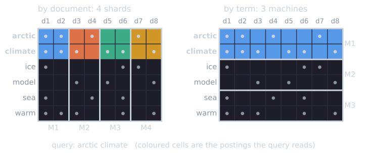
The trade-offs between them:
| Document partitioning | Term partitioning | |
|---|---|---|
| Machines involved per query | All shards | Only those holding the query's terms |
| Work per machine per query | Small: a short postings list for every query term | Large for common terms: entire postings lists |
| Data moved between machines | Only each shard's top $k$ results | Whole postings lists, or partial results passed along |
| Load balance | Even, if documents are spread randomly | Uneven: machines holding popular terms become hot spots |
| Collection statistics | Each shard sees only local document frequencies | Each term's statistics are complete on one machine |
| Adding documents | Add to one shard or add a shard | Touches the postings of many terms on many machines |
Term partitioning looks efficient, because a two-word query involves only two machines. In practice its costs dominate. A rough count of bytes shows why. In the billion-document collection above, take a query whose two terms occur in 1 percent and 0.1 percent of documents. Their postings lists hold 10 million and 1 million docIDs, about 11.6 MB and 1.2 MB at variable-byte rates. Under term partitioning, the shorter list must travel to the machine holding the longer one, or both to a third, and both lists are read in full. Under document partitioning into the 10 shards sized above, each shard returns its top 10 results, at 12 bytes each for a docID and a score, a total of $10 \times 10 \times 12 = 1{,}200$ bytes, and each shard reads only its tenth of each list. The postings list for a common term can be enormous, and it must be transferred and combined, so the machines holding popular terms become bottlenecks. Moffat, Webber, Zobel, and Baeza-Yates (2007) showed that pipelined designs can mitigate this, but large web engines have generally chosen document partitioning (Barroso, Dean, and Hölzle, 2003; Dean, 2009). Document partitioning also isolates failures well: if one shard does not respond, the query can still be answered from the others. The loss in recall is, on average, about the share of the collection that shard holds, but for a particular query it can be large, for example when the one page a navigational query seeks is on the missing shard.
Document partitioning has one subtle cost. Ranking functions such as TF-IDF and BM25 depend on collection-wide statistics such as document frequency and average document length. A shard that computes them over its own documents will score slightly differently from its neighbors, and the merged ranking will compare scores that are not quite comparable. If documents are assigned to shards at random and each shard is large, local statistics are close to the global ones for most terms and the error is small. Rare terms are the exception: a term that occurs in a few dozen documents can have very different document frequencies on different shards.
The size of the effect can be measured. Splitting the 10,788 stories of Reuters-21578 at random into shards and comparing each shard's $\log_{10}(N_s/\text{df}_s)$ with the global $\log_{10}(N/\text{df})$, for every term on every shard where it occurs, gives the following median absolute differences (computed by tools/experiments/foundations/shard_statistics.py; median over 30 random splits, whose interquartile ranges are 0.002 or narrower; rounded to two places):
| Global df of the term | Terms | Median idf error, 8 shards | Median idf error, 64 shards |
|---|---|---|---|
| 1 to 9 | 23,559 | 0.60 | 1.33 |
| 10 to 99 | 4,476 | 0.14 | 0.37 |
| 100 to 999 | 1,055 | 0.05 | 0.14 |
| 1,000 or more | 97 | 0.02 | 0.04 |
For scale, idf on this collection runs from 4.03 for a word in a single story down to below 1 for words in more than a tenth of the stories. With eight shards, a term in a few hundred stories, with an idf near 1.5, strays by about 0.05 on a typical shard, a few percent. A term in one story sits on one shard, where its local idf is about $\log_{10}(10{,}788/8)$ instead of $\log_{10}(10{,}788)$, smaller by $\log_{10} 8 \approx 0.90$. A term in two stories that land on different shards is off by $\log_{10} 4 \approx 0.60$, which is the median for the rarest band. The error grows with the number of shards, because each shard is a smaller sample of the collection. When precision matters, the global statistics are computed periodically and distributed to every shard.
Replication
Partitioning makes the index fit. Replication makes the service fast and reliable. Each shard is copied onto several machines, and a load balancer sends each query to one replica of each shard. Doubling the number of replicas roughly doubles the number of queries the system can serve. Replicas also provide fault tolerance: when a machine fails, its queries go to another replica of the same shard. A large deployment can therefore be pictured as a grid, with shards in one dimension and replicas in the other. The number of shards is set mainly by the size of the index, and the number of replicas by the query load and the level of fault tolerance required.
Caching
Query traffic is very uneven. A small number of queries are issued over and over, while a large fraction of distinct queries are seen only once. That distribution makes caching effective. Baeza-Yates and colleagues (2007) analyzed caching at two levels:
- Result caches store the final results page for a query. When the same query arrives again, the engine returns the stored page without consulting the index at all. This saves the most work per hit, but it helps only with repeated queries. The cache key must include everything else that changes the results, such as language, location, personalization, and, in enterprise search, the user's access rights.
- Postings caches store the postings lists of frequently used terms in memory. A new query made of common terms is then answered without reading those lists from disk. Hits are less valuable than result-cache hits, but much more frequent, because many distinct queries share common terms.
Two refinements matter in practice. A cache can be divided into a static part, filled from historical logs with queries that are always popular, and a dynamic part, managed by a replacement policy that tracks what is popular now (Fagni, Perego, Silvestri, and Orlando, 2006). And because the index changes, a cached result goes stale. Each entry needs an expiry policy, which sets the balance between saving work and showing results that no longer reflect the index.
Memory has also replaced disk for most serving. Dean (2009) described Google moving its serving index entirely into memory early in the 2000s, once the combined memory of its machines could hold it, which removed disk seeks from the query path. Many large deployments now serve most or all of the index from memory or from solid-state storage.
Doing less work per query
Even with partitioning and caching, scoring every document that matches a query is wasteful. Most of them will never be shown. Several techniques avoid that work.
Tiered indexes. The index is divided by document quality. The first tier contains a small fraction of high-quality pages and is consulted for every query. Lower tiers are consulted only if the first tier returns too few good results (Manning, Raghavan, and Schütze, 2008, §7.2.1). Because most queries are answered well from the first tier, most of the index sits idle for most queries. The saving is approximate: a lower-tier page that would have ranked highly is never considered when the first tier suffices.
Early termination. If postings are ordered so that documents likely to score highly come first, a query can stop reading once its top $k$ results cannot change. Algorithms such as WAND (Broder, Carmel, Herscovici, Soffer, and Zien, 2003) maintain an upper bound on the score each term can contribute, and skip documents that cannot reach the current $k$-th best score. When the bounds are valid for the full scoring function, the technique produces exactly the same top $k$ as scoring everything, at a fraction of the cost. Broder and colleagues also made the pruning threshold adjustable: raising it above the current $k$-th best score skips more documents and saves more work, at the risk of losing some true top-$k$ results. Tonellotto, Macdonald, and Ounis (2018) survey these methods.
Multi-stage ranking. Ranking is organized as a cascade. A cheap first stage, such as BM25 over the inverted index, selects perhaps a thousand candidates from millions of matches. A second stage applies a learned model over hundreds of features to those candidates. A final stage applies the most expensive model, such as a neural model that reads the query and the document text together, to the top few dozen. Each stage reduces the candidate set for the next, so expensive computation is spent only on documents likely to be shown (Wang, Lin, and Metzler, 2011). This structure is why classical models remain in production even where neural models are more accurate: the neural models are affordable only because a cheaper first stage, usually a classical model, has already discarded almost every document.
Tail latency
A query on a document-partitioned index waits for the slowest shard. If each of a hundred shards independently responds within its usual time 99 percent of the time, the probability that all hundred respond in time is $0.99^{100} \approx 0.37$. Most queries are therefore slowed by at least one straggler. Dean and Barroso (2013) called this the tail at scale: at high fan-out, rare delays on individual machines become common delays for the service. This is one cost of dividing an index into more shards than it needs: each additional shard is another chance for a query to wait. In practice delays are also partly correlated, through shared networks and machines, so the independent model is an illustration rather than a prediction.
The general form follows from the same reasoning. If each of $S$ shards is slow with probability $p$, independently, the query escapes delay only if every shard is fast, so
$$P(\text{query slow}) = 1 - (1 - p)^S.$$
For small $p$ this is close to $Sp$ while $Sp$ is small, and it passes one half when $S \approx 0.69/p$: at about 69 shards for $p = 1/100$, 693 for $p = 1/1{,}000$, and 6,931 for $p = 1/10{,}000$ (computed by tools/experiments/foundations/scale_arithmetic.py). Dean and Barroso (2013, pp. 76–77) plot this curve for a server that usually answers in 10 ms but takes a second one time in a hundred: with 100 such servers, 63 percent of requests take more than a second, and even if only one request in 10,000 is slow, a service with 2,000 servers sees almost one request in five take more than a second.
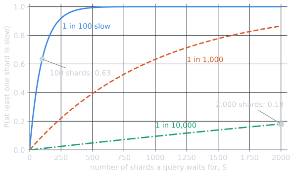
Measurements from a real service agree in shape. Dean and Barroso (2013, p. 77, Table 1) report a Google service in which a root server fans a request out to a very large number of leaf servers. At the 99th percentile, a single randomly chosen leaf finishes in 10 ms, 95 percent of the leaves finish in 70 ms, and all of them in 140 ms. Waiting for the slowest 5 percent of leaves accounts for half of that 140 ms.
The remedies accept some redundancy. A hedged request sends a query to a second replica if the first has not answered within a short delay, and uses whichever answer arrives first. Waiting before hedging keeps the cost down: if the second request is sent only after the first has been outstanding longer than the 95th-percentile latency for its class, only about 5 percent of requests are duplicated. In a Google benchmark that read 1,000 values spread over 100 servers, hedging after 10 ms cut the 99.9th-percentile latency from 1,800 ms to 74 ms while sending only 2 percent more requests (Dean and Barroso, 2013, p. 77). An idealized calculation shows why the gain is so large. If the two replicas were slow independently, each with probability $p$, a hedged shard would be slow only when both were, with probability $p^2$. For $p = 1/100$ that is $1/10{,}000$, and the probability that a 100-shard query is slow falls from 0.63 to 0.01. Real delays are partly correlated, so the gain is smaller, but the benchmark shows it can still be large. A deadline lets the broker return results without a shard that is too slow, accepting some loss in recall for that query in exchange for a predictable response time. Engines also monitor latency at high percentiles, such as the 99th, rather than at the average, because the average hides exactly the delays that users notice.
Keeping the index fresh
The index is a snapshot. Between the moment a page is crawled and the moment the index containing it goes into service, the page may change, and new pages appear that the index does not contain. How long that lag lasts depends on how the index is built.
The traditional approach rebuilt the index in large batches. The crawled collection was processed into a new index over hours or days, and the new index replaced the old one in service. Batch rebuilding is simple and efficient, but every page in the index is at least as old as the most recent rebuild, and any change after that rebuild's crawl must wait for the next one. For a news event, that is far too old.
Modern engines combine a large main index, rebuilt or merged periodically, with small indexes of recent documents that are updated continuously. A query is answered from both, and the small indexes are merged into the main one in the background, the approach called logarithmic merging in index construction (Manning, Raghavan, and Schütze, 2008, §4.5). Google's move to incremental indexing in 2010 relied on a system for processing updates to individual pages as they were crawled, rather than recomputing over the whole collection (Peng and Dabek, 2010). Freshness also depends on the crawler, since a page cannot be indexed until it has been fetched again. Deciding how often to revisit each page is a central problem in web crawling.
Different parts of the collection need different freshness. A news site's home page changes many times a day and an academic paper hardly ever. Engines allocate crawling and indexing resources accordingly, and use the age of the indexed copy as one of the inputs to ranking for queries that require fresh results.
The same ideas at smaller scale
Open-source search servers such as Elasticsearch and Solr, both built on the Lucene library, implement the same architecture on a small scale. An index is divided into shards that hold disjoint sets of documents, each shard has configurable replicas, a coordinating node scatters each query to the shards and gathers their results, and new documents are written to small segments that are merged in the background. Lucene's segments and background merges apply the merge-based dynamic indexing described in the textbook. A segment is not a shard: each shard is a complete Lucene index, which usually consists of many segments. An organization indexing a few million documents may need only a few machines, but it still decides how many shards to use, how many replicas to keep, how fresh the index must be, and whether to compute collection statistics per shard or globally.
What does not carry over from the web is the volume of behavioral data and the link graph. Those differences shape ranking more than infrastructure, and they are the subject of enterprise, personal, and product search.
Summary
Scale changes the engineering of retrieval but not its logic. Partitioning makes the index fit, replication handles query load and failure, caching exploits the repetition in query traffic, and tiering, early termination, and staged ranking reduce the work per query. Each technique trades something for speed: memory for disk reads, redundant computation for predictable latency, a little recall for a guaranteed response time, and absolute freshness for efficient rebuilding. The architecture article describes a single pipeline. A production engine runs thousands of copies of pieces of that pipeline in parallel, organized so that the user still sees a single, consistent ranked list.
References
- Baeza-Yates, R., Gionis, A., Junqueira, F., Murdock, V., Plachouras, V., and Silvestri, F. (2007). The impact of caching on search engines. In Proceedings of SIGIR 2007, 183–190.
- Barroso, L. A., Dean, J., and Hölzle, U. (2003). Web search for a planet: The Google cluster architecture. IEEE Micro, 23(2), 22–28.
- Broder, A. Z., Carmel, D., Herscovici, M., Soffer, A., and Zien, J. (2003). Efficient query evaluation using a two-level retrieval process. In Proceedings of CIKM 2003, 426–434.
- Dean, J. (2009). Challenges in building large-scale information retrieval systems. Keynote, WSDM 2009.
- Dean, J., and Barroso, L. A. (2013). The tail at scale. Communications of the ACM, 56(2), 74–80.
- Fagni, T., Perego, R., Silvestri, F., and Orlando, S. (2006). Boosting the performance of Web search engines: Caching and prefetching query results by exploiting historical usage data. ACM Transactions on Information Systems, 24(1), 51–78.
- Manning, C. D., Raghavan, P., and Schütze, H. (2008). Introduction to Information Retrieval, sections 2.4.2, 4.5, 7.1–7.2, and 20.3, and chapter 5. Cambridge University Press.
- Moffat, A., Webber, W., Zobel, J., and Baeza-Yates, R. (2007). A pipelined architecture for distributed text query evaluation. Information Retrieval, 10(3), 205–231.
- Peng, D., and Dabek, F. (2010). Large-scale incremental processing using distributed transactions and notifications. In Proceedings of OSDI 2010, 251–264.
- Tonellotto, N., Macdonald, C., and Ounis, I. (2018). Efficient query processing for scalable web search. Foundations and Trends in Information Retrieval, 12(4–5), 319–500.
- Wang, L., Lin, J., and Metzler, D. (2011). A cascade ranking model for efficient ranked retrieval. In Proceedings of SIGIR 2011, 105–114.