In any large body of text, a few words do most of the work. If the frequencies of the 400,000 distinct terms in a collection followed Zipf's law exactly, the single most frequent term would account for about 7 percent of all tokens. The ten most frequent would account for about 22 percent, and the hundred most frequent for nearly 39 percent. Half of all the tokens in the collection would come from just 474 terms, about a tenth of a percent of the vocabulary. The other 399,500 terms would share the remaining half, and most of them would occur only a handful of times.
Two empirical regularities describe this situation. Zipf's law describes how frequencies are distributed across the vocabulary. Heaps' law describes how the vocabulary grows as the collection grows. Neither is exact, but both hold well enough across languages and collections to guide the design of nearly every component in this topic: which words to treat as stop words, how large the dictionary will become, and why compression works.
Two kinds of frequency
Two frequency counts recur throughout retrieval, and they behave differently:
- The collection frequency $\mathit{cf}_t$ of a term $t$ is the total number of times it occurs in the collection, counting every token.
- The document frequency $\mathit{df}_t$ is the number of documents that contain $t$ at least once.
They can diverge sharply. Manning, Raghavan, and Schütze (2008, §6.2.1) give an example from the Reuters collection. Try and insurance have almost the same collection frequency, 10,422 and 10,440 occurrences. But try occurs in 8,760 documents and insurance in only 3,997. Try is spread thinly across many documents, while insurance is concentrated in fewer documents that use it repeatedly, which is the pattern of a word that indicates what a document is about. Document frequency captures that difference and collection frequency does not, which is why inverse document frequency is computed from $\mathit{df}$. Zipf's law is usually stated in terms of collection frequency.
The rest of this article measures both laws on one real collection, so it helps to see the two counts there first. Reuters-21578 (Lewis, 1997) is an older and much smaller Reuters newswire collection than RCV1: in the version distributed with the NLTK toolkit it has 10,788 news stories from 1987. Lowercasing the text and taking every maximal run of letters as a token gives 1,330,267 tokens and 29,187 distinct terms. Some of its terms (ratios rounded to one decimal):
| Term | $\mathit{cf}$ | $\mathit{df}$ | $\mathit{cf}/\mathit{df}$ |
|---|---|---|---|
| the | 69,277 | 6,951 | 10.0 |
| said | 25,383 | 6,784 | 3.7 |
| mln | 18,623 | 4,849 | 3.8 |
| dlrs | 12,417 | 4,226 | 2.9 |
| oil | 3,272 | 1,038 | 3.2 |
| zinc | 115 | 50 | 2.3 |
The ratio $\mathit{cf}/\mathit{df}$ is the average number of occurrences in the documents that contain the term. The occurs in 64 percent of the stories and about ten times in each. Said is nearly as widespread, since almost every news story reports what someone said, but appears fewer times per story. Mln (million) and dlrs (dollars) are the house abbreviations of a financial newswire. A term's rank by $\mathit{cf}$ and its rank by $\mathit{df}$ can therefore differ, and the choice matters whenever a list of "most common words" is drawn up.
Zipf's law
Sort the terms of a collection by collection frequency, so that the most frequent has rank 1, the next rank 2, and so on. George Kingsley Zipf (1949) observed that frequency is roughly inversely proportional to rank:
$$\mathit{cf}_i \propto \frac{1}{i},$$
where $\mathit{cf}_i$ is the collection frequency of the term at rank $i$. The second most frequent term occurs about half as often as the first, the third about a third as often, and so on. Taking logarithms gives $\log \mathit{cf}_i = \log c - \log i$ for some constant $c$, so on a plot with logarithmic axes the terms fall close to a straight line with slope $-1$. Real collections deviate from the line at both ends, with the very top ranks and the long tail usually falling below it. Mandelbrot proposed a better-fitting generalization, $\mathit{cf}_i = P(i + \rho)^{-B}$, with parameters fitted to each collection. The simple form is accurate enough for reasoning about index design (Manning, Raghavan, and Schütze, 2008, §5.1.2).
Where the numbers above come from
If $\mathit{cf}_i = c/i$ for a vocabulary of $M$ terms, the total number of tokens is
$$T = \sum_{i=1}^{M} \frac{c}{i} = c \, H_M,$$
where $H_M = 1 + \tfrac{1}{2} + \dots + \tfrac{1}{M}$ is the $M$-th harmonic number, approximately $\ln M + 0.577$. The fraction of all tokens contributed by the top $k$ terms is therefore $H_k / H_M$. For $M = 400{,}000$, $H_M \approx 13.48$, and:
| Top $k$ terms | $H_k$ | Share of all tokens |
|---|---|---|
| 1 | 1.00 | 7.4% |
| 10 | 2.93 | 21.7% |
| 100 | 5.19 | 38.5% |
| 1,000 | 7.49 | 55.5% |
The cumulative share first reaches one half at rank 474. These figures describe an idealized collection, but real ones are similar: a short list of function words such as the, of, and, and to accounts for a large fraction of all text.
Two steps in this calculation deserve a word. First, the constant $c$ is not a free parameter once the vocabulary is fixed: setting the total to $T$ forces $c = T / H_M$, so the most frequent term's share of the collection is $1/H_M$. A larger vocabulary means a larger $H_M$ and a smaller share for every term. Second, the approximation $H_M \approx \ln M + 0.577$ comes from comparing the sum with the integral $\int_1^M dx/x = \ln M$. The sum overshoots the integral by a nearly constant amount, which tends to the Euler–Mascheroni constant $\gamma \approx 0.5772$ as $M$ grows. For $M = 400{,}000$ the approximation gives $12.899 + 0.577 = 13.476$, the same as the exact sum to three decimals.
Zipf's law on a real collection
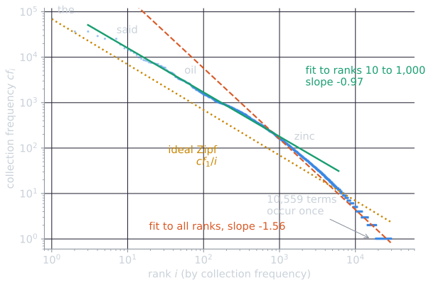
The Reuters-21578 collection introduced above makes a useful test. Sorting its 29,187 terms by collection frequency and plotting frequency against rank on logarithmic axes gives the figure below.
Three features of the plot recur in nearly every collection:
- The middle is close to Zipf. A least-squares line through ranks 10 to 1,000 has slope $-0.974$. Over that range the product $i \cdot \mathit{cf}_i$ is roughly constant, which is what $\mathit{cf}_i = c/i$ says. Divided by $T$ to make it a share, the product is $0.112$ for said (rank 6), $0.116$ for oil (rank 47), and $0.114$ for zinc (rank 1,314).
- The head is flatter. The has a share of $0.052$, not $0.11$: the most frequent words occur less often than a line through the middle predicts.
- The tail is steeper. Beyond about rank 1,000 the points fall away faster than slope $-1$ (a fit to ranks 3,000 to 10,000 has slope $-1.69$), ending in horizontal steps at frequencies 3, 2, and 1, since many terms share each small integer frequency. These tied terms are so numerous that a line fitted through every point is dominated by them and has slope $-1.557$. That is why the fit in the code below depends so much on which ranks it includes.
The cumulative shares show the same picture. The ideal column uses $H_k / H_M$ with the collection's own vocabulary size, $M = 29{,}187$, for which $H_M = 10.859$ (all shares rounded to one decimal):
| Top $k$ terms | Ideal Zipf | Reuters-21578 |
|---|---|---|
| 1 | 9.2% | 5.2% |
| 10 | 27.0% | 22.3% |
| 100 | 47.8% | 49.1% |
| 1,000 | 68.9% | 79.2% |
The real head is lighter than the ideal one, and the real tail is lighter still, so the middle ranks carry more of the text than Zipf predicts. Half of all tokens come from the 109 most frequent terms, 0.37 percent of the vocabulary.
The long tail
Zipf's law also predicts how many terms are rare. If a term's rank is approximately $c/f$ when its frequency is $f$, then the number of terms with frequency exactly $f$ is approximately
$$\frac{c}{f} - \frac{c}{f+1} = \frac{c}{f(f+1)}.$$
The rarest terms, with frequency 1, sit at rank about $c$, so the vocabulary has about $c$ terms, and the proportion of the vocabulary occurring exactly $f$ times is about $1/(f(f+1))$: one half for $f = 1$, one sixth for $f = 2$, one twelfth for $f = 3$. This is an idealized estimate. Real frequencies are integers, and the tail of a finite collection is shaped by sampling and by text processing, so measured proportions differ. Croft, Metzler, and Strohman (2010, §4.2) use this argument to conclude that about half of the distinct terms in a large collection occur only once. Such terms are called hapax legomena. They include genuine rare words, but also names, misspellings, codes, and tokenization accidents, and they make up much of the dictionary while contributing very little to the postings.
The derivation in the first line deserves unpacking. Zipf's law gives frequency as a function of rank. Turned around, the rank of a term with frequency $f$ is about $c/f$, which is also the number of terms whose frequency is at least $f$, since they are exactly the terms ranked above it. The terms with frequency exactly $f$ are those with frequency at least $f$ minus those with frequency at least $f + 1$, which gives the difference above. Reuters-21578 can be compared with the prediction directly (proportions of the vocabulary, rounded to three decimals):
| Frequency $f$ | Terms | Share of vocabulary | Ideal $1/(f(f+1))$ |
|---|---|---|---|
| 1 | 10,559 | 0.362 | 0.500 |
| 2 | 4,212 | 0.144 | 0.167 |
| 3 | 2,347 | 0.080 | 0.083 |
| 4 | 1,639 | 0.056 | 0.050 |
| 5 | 1,081 | 0.037 | 0.033 |
From $f = 3$ on, the prediction is close. At $f = 1$ it is too high, the same shortfall seen in the 36 percent of this wiki's terms that occur once, reported below. The 10,559 hapax legomena are 36 percent of the dictionary but only 0.8 percent of the tokens. A random sample of 25 of them shows the mixture described above: misspellings (certian, microgrpahics), surnames and company names (haarmann, jepson, sobey), ticker-like codes (cvsi, rhds), and ordinary but uncommon words (augers, custody, unflappable).
Consequences for indexing
The shape of the distribution explains several design decisions:
- Stop words. The handful of terms at the top of the ranking are mostly function words, occur in nearly every document, and have the longest postings lists. Removing them was historically the cheapest way to shrink an index. The stop words article discusses why that trade is less attractive today.
- Luhn's significance band. Hans Peter Luhn (1958) argued that the words most useful for representing a document's content lie in the middle of the frequency range. The most frequent words are too common to discriminate between documents, and the rarest are too infrequent to be reliable. Term weighting schemes such as TF-IDF later replaced fixed frequency cut-offs with continuous weights that express the same idea.
- Skewed postings. A few postings lists are enormous and most are tiny. In Reuters-21578, the 97 terms that occur in at least 1,000 stories hold 33 percent of all postings, while the 12,769 terms that occur in exactly one story hold under 2 percent. Compression methods are designed around this: the long lists of frequent terms contain many small gaps between document numbers, which can be stored in very few bits. The index compression article measures the effect on the same collection.
Heaps' law
How many distinct terms should a collection of a given size be expected to contain? Harold Heaps (1978) described the relationship that now bears his name:
$$M = k \, T^{b},$$
where $M$ is the vocabulary size, $T$ is the number of tokens in the collection, and $k$ and $b$ are parameters fitted to the collection. Typical values are $30 \le k \le 100$ and $b \approx 0.5$ (Manning, Raghavan, and Schütze, 2008, §5.1.1). On logarithmic axes this too is a straight line, with slope $b$.
For the Reuters RCV1 collection, Manning, Raghavan, and Schütze fit $k = 44$ and $b = 0.49$. For the first 1,000,020 tokens the law predicts
$$M = 44 \times 1{,}000{,}020^{0.49} \approx 38{,}323$$
distinct terms. The actual count is 38,365, a close fit. Extrapolating to the whole collection, which the textbook describes as about $10^{8}$ tokens, predicts
$$M = 44 \times (10^{8})^{0.49} \approx 365{,}976$$
terms, close to the collection's actual vocabulary of about 400,000 terms.
Heaps' law on a real collection
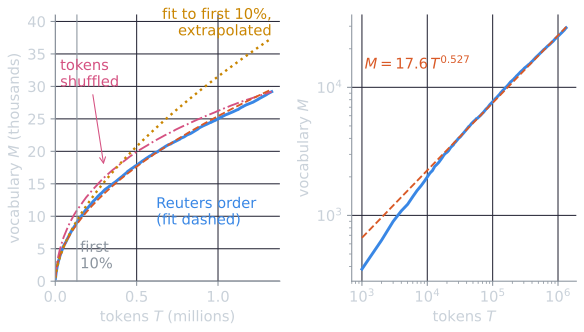
Reading the Reuters-21578 stories in order of their Reuters identifiers, which is roughly the order in which they were filed, and recording the vocabulary size after every 1,000 tokens gives 1,330 checkpoints. A least-squares line through their logarithms gives
$$M = 17.6 \, T^{0.527}.$$
The exponent is close to the textbook's typical value. The constant is below the typical range of 30 to 100. The two parameters are not independent: a line in log space that is slightly steeper must start lower to pass through the same points, so a larger $b$ comes with a smaller $k$, as the fit to part of the collection below also shows. With $T = 1{,}330{,}267$ the fit predicts $17.6 \times 1{,}330{,}267^{0.527} \approx 29{,}550$ terms, against 29,187 observed (the computation uses the unrounded parameters, $k = 17.62$ and $b = 0.5267$).
What the fitted law predicts is the useful part. Since $M$ grows as $T^{b}$, multiplying the collection by a factor $m$ multiplies the vocabulary by $m^{b}$:
| Collection size | Tokens | Predicted vocabulary | Growth factor $m^{0.527}$ |
|---|---|---|---|
| Reuters-21578 | 1.33 million | 29,550 | 1 |
| twice as large | 2.66 million | 42,567 | 1.44 |
| ten times | 13.3 million | 99,341 | 3.36 |
| a hundred times | 133 million | 333,959 | 11.30 |
A hundred times the text yields only about eleven times the vocabulary. This kind of extrapolation is also where the law is weakest. Fitting only the first 10 percent of the collection (133,000 tokens) gives $k = 7.6$ and $b = 0.603$, which predicts 37,442 terms for the whole collection instead of the 29,187 observed. The exponent fitted on a small sample is too large because the curve is not quite straight on logarithmic axes. Its slope is steeper over the first few thousand tokens, when even common words are still appearing for the first time, and flattens as the collection grows, as the right-hand panel of the figure shows. Extrapolations over two orders of magnitude, like the RCV1 one above, deserve the same caution even when they turn out well.
The order of the text matters as well. Shuffling all the tokens of the collection into a random order, which destroys the grouping of words into stories and of stories into weeks of news, and refitting gives $b = 0.465$ (median over 30 shuffles with different random seeds, interquartile range 0.463 to 0.467). Halfway through the shuffled stream the vocabulary already holds a median of 22,387 terms, against 20,553 in the original order. In real text, rare words cluster: a story about a company names it several times, and a news event introduces its vocabulary at the time it happens. New terms are therefore revealed later than random sampling would reveal them, and the real curve keeps climbing longer.
Consequences for indexing
The important property of Heaps' law is that $b < 1$ but $b > 0$. Vocabulary grows more slowly than the collection, roughly with its square root, but under the law it never stops growing. Doubling a collection's size increases its vocabulary by a factor of about $2^{0.5} \approx 1.4$. New names, products, technical terms, and misspellings keep appearing however much text has already been seen. This has practical consequences:
- Dictionary size. The dictionary of a large collection does not level off at the size of a natural-language vocabulary. A web-scale index has hundreds of millions of distinct terms, and the dictionary must be designed to hold them, which is one motivation for dictionary compression.
- Dynamic indexes. A system that adds documents over time will keep encountering terms it has never seen, so an indexer cannot fix its vocabulary in advance. The index construction algorithms are designed with this in mind.
- Out-of-vocabulary queries. A query term absent from the dictionary is common, not exceptional. Systems respond with spelling correction, or, in neural models, with the subword tokenization described earlier.
Measuring them on a collection
Both laws are straight lines on logarithmic axes, so their parameters can be estimated by linear regression on the logarithms. A least-squares fit in log space is a quick diagnostic, not a rigorous estimate of a power-law exponent: its result depends on which ranks are included, and the many tied low-frequency terms in the tail pull on the slope. The following code fits both to a list of texts large enough to give several Heaps' law checkpoints:
import re
from collections import Counter

import numpy as np


def tokens(text):
    return re.findall(r"[a-z]+", text.lower())


def zipf_slope(counts):
    freqs = np.array(sorted(counts.values(), reverse=True), dtype=float)
    ranks = np.arange(1, len(freqs) + 1)
    slope, _ = np.polyfit(np.log10(ranks), np.log10(freqs), 1)
    return slope


def heaps_fit(stream, every=1000):
    seen, xs, ys = set(), [], []
    for i, tok in enumerate(stream, 1):
        seen.add(tok)
        if i % every == 0:
            xs.append(i)
            ys.append(len(seen))
    b, log_k = np.polyfit(np.log10(xs), np.log10(ys), 1)
    return 10 ** log_k, b


texts = [...]  # the documents, as a list of strings
stream = [t for text in texts for t in tokens(text)]
counts = Counter(stream)
print(zipf_slope(counts), heaps_fit(stream))
Applied to the articles of this wiki, at a point when it held 28 articles and 51,444 tokens, the code found 4,985 distinct terms. The ten most frequent were the, and, a, of, in, is, to, that, for, and it, all function words. 36 percent of the terms occurred exactly once. The fitted Zipf slope was $-1.18$, close to the ideal $-1$. Heaps' law fit with $k \approx 3.8$ and $b \approx 0.67$, outside the typical ranges given above, which is what one should expect from a collection this small and this uniform in subject and style. Parameters fitted on a small sample are poor guides to a large collection. That is one reason textbooks quote values from collections such as RCV1.
How the two laws relate
Zipf's law and Heaps' law are not independent. A vocabulary with a long tail of rare terms is exactly a vocabulary that keeps growing, because every new stretch of text draws some terms from that tail for the first time. Under suitable assumptions, Heaps' law can be derived from a Zipf-like frequency distribution (van Leijenhorst and van der Weide, 2005).
A rough version of the argument shows where the exponent comes from. Suppose text is generated by drawing each token independently, with the term of rank $r$ drawn with probability $p_r = r^{-s}/Z$, where $s > 1$ is the Zipf exponent and $Z$ makes the probabilities sum to one. After $T$ tokens, a term of rank $r$ is expected to have occurred $T p_r$ times.
- Terms with $T p_r$ well above 1 have almost certainly been seen. Terms with $T p_r$ well below 1 have almost certainly not. The vocabulary is therefore roughly the set of ranks up to the point $r^{*}$ where $T p_{r^{*}} = 1$.
- Solving $T (r^{*})^{-s} / Z = 1$ gives $r^{*} = (T/Z)^{1/s}$.
- The terms beyond $r^{*}$ that have been seen anyway contribute about $\sum_{r > r^{*}} T p_r \approx \frac{T}{Z} \int_{r^{*}}^{\infty} x^{-s}\,dx = \frac{r^{*}}{s-1}$, which has the same form, so they change the constant but not the exponent.
So $M \approx k\,T^{1/s}$: Heaps' law, with $b = 1/s$. A steeper Zipf curve, in which rare terms are rarer, gives slower vocabulary growth. A simulation checks the argument: drawing a million tokens from such a distribution over two million ranks and fitting Heaps' law as above gives $b = 0.661$ for $s = 1.5$ and $b = 0.502$ for $s = 2$ (medians over 30 seeds, interquartile ranges 0.658 to 0.664 and 0.495 to 0.507), against predictions of 0.667 and 0.5. Real text is not drawn independently, as the shuffling experiment showed, and its rank-frequency curve is not one straight line, so the relation explains the form of Heaps' law better than it predicts a particular collection's exponent.
Together they describe the basic statistical situation every indexer faces. A small set of terms accounts for most of the text and the longest postings lists. A vast and still-growing set of rare terms accounts for most of the vocabulary. The inverted index, its construction, and its compression are all shaped by having to handle both at once.
References
- Croft, W. B., Metzler, D., and Strohman, T. (2010). Search Engines: Information Retrieval in Practice, section 4.2. Addison-Wesley.
- Heaps, H. S. (1978). Information Retrieval: Computational and Theoretical Aspects. Academic Press.
- Lewis, D. D. (1997). Reuters-21578 text categorization test collection, distribution 1.0.
- Luhn, H. P. (1958). The automatic creation of literature abstracts. IBM Journal of Research and Development, 2(2), 159–165.
- Manning, C. D., Raghavan, P., and Schütze, H. (2008). Introduction to Information Retrieval, sections 5.1 and 6.2. Cambridge University Press.
- van Leijenhorst, D. C., and van der Weide, T. P. (2005). A formal derivation of Heaps' Law. Information Sciences, 170(2–4), 263–272.
- Zipf, G. K. (1949). Human Behavior and the Principle of Least Effort. Addison-Wesley.