A user searching for "stanford university" wants documents about the university. A document containing the sentence The inventor Stanford Ovshinsky never went to university contains both words and satisfies stanford AND university, but it is not about the institution (Manning, Raghavan, and Schütze, 2008, §2.4). The Boolean model as described so far cannot tell the difference, because its postings record only which documents contain each term, not where.
Phrase queries, usually marked with quotation marks, ask for words in a specific sequence. Proximity queries ask for words within some distance of each other, in either order. Many queries name things, such as New York, machine learning, or Department of Defense, whose words mean something only together. This article describes the two ways of extending the index to support such queries and how production systems combine them.
Biword indexes
The simplest approach treats each pair of consecutive words as a single term. The text friends Romans countrymen produces the biwords friends romans and romans countrymen, each with its own postings list in the dictionary. A two-word phrase query becomes a single dictionary lookup.
A longer phrase is broken into overlapping biwords and evaluated as their conjunction. The query "stanford university palo alto" becomes
"stanford university" AND "university palo" AND "palo alto"
This can produce false positives. A document might contain stanford university in one paragraph, university palo in another, and palo alto in a third, without ever containing the four-word phrase. The documents retrieved must then be checked against their text to confirm that the full phrase occurs.
Biword indexes have two further costs. The dictionary grows enormously, since the number of distinct word pairs in a collection far exceeds the number of distinct words. And a biword index cannot answer proximity queries at all. One refinement indexes extended biwords, pairs of nouns separated by any number of function words, identified by part-of-speech tagging. Cost overruns on a power plant is then indexed as cost overruns, overruns power, and power plant, so queries match despite intervening words (Manning, Raghavan, and Schütze, 2008, §2.4.1). The approach is rarely used alone, but indexing selected word pairs survives as part of combined schemes, described below.
How large, and how wrong?
Both costs can be measured on a real collection. The Cranfield collection has 1,400 abstracts of aerodynamics papers. Tokenized into lowercase words, with no stop list and no stemming, it has:
| Quantity | Count |
|---|---|
| Tokens (word occurrences) | 243,353 |
| Distinct words | 7,472 |
| Distinct biwords | 75,583 |
| Distinct three-word phrases | 157,304 |
The biword dictionary is ten times the size of the word dictionary, even for this small, specialized collection, and the dictionary of three-word phrases is twice as large again.
To measure false positives, every three-word phrase that occurs in the collection was run as a query in two ways: as the conjunction of its two biwords, and exactly. Summed over all 157,304 phrases, the biword conjunctions retrieve 298,298 documents, of which 216,055 contain the phrase. The other 82,243, 27.6 percent of what the biword index retrieves, are false positives. Nearly all of them, 98.4 percent, come from phrases containing a stop word, which pairs with almost anything: of the results occurs in 26 abstracts, but of the and the results co-occur in 235. Phrases made only of content words fare far better, with 3.0 percent false positives, but are not immune. mach number range occurs in 31 abstracts, while mach number and number range co-occur in 36. (Stop words here are the 33-word list this site's search uses.) These figures come from tools/experiments/boolean/phrase_queries.py.
Positional indexes
The standard solution stores, in each posting, the positions at which the term occurs in the document. A positional index entry has the form
term: df
    docID: tf; position, position, ...
    docID: tf; position, position, ...
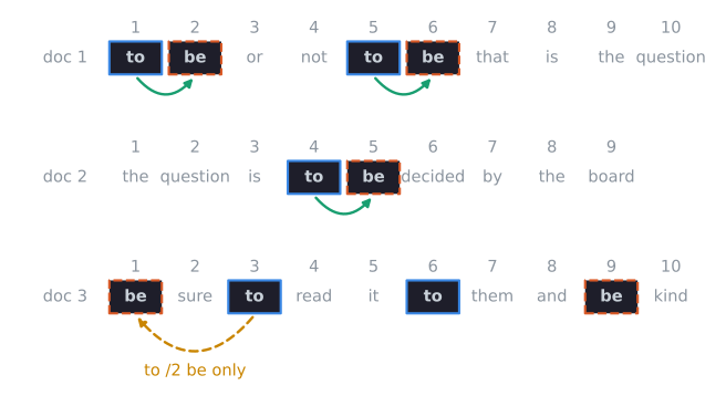
where the term frequency $\mathit{tf}$ is simply the number of positions listed. Consider three short documents, with positions counted in words from 1:
| docID | Text |
|---|---|
| 1 | to be or not to be that is the question |
| 2 | the question is to be decided by the board |
| 3 | be sure to read it to them and be kind |
The positional postings for to and be are:
to:  doc 1: 1, 5    doc 2: 4    doc 3: 3, 6
be:  doc 1: 2, 6    doc 2: 5    doc 3: 1, 9
Answering a phrase query
To find "to be":
- Intersect the two terms' document lists, as in an ordinary AND, to find documents containing both terms: 1, 2, and 3.
- In each such document, look for a position of be exactly one greater than a position of to.
In document 1, to at 1 is followed by be at 2, and to at 5 by be at 6, giving two occurrences. In document 2, to at 4 is followed by be at 5. In document 3, to appears at 3 and 6 and be at 1 and 9, never adjacent. The answer is documents 1 and 2. Unlike the biword approach, this result is exact, with no false positives to filter.
Step 2 is itself a merge. Both position lists are sorted, so instead of comparing every pair, the algorithm walks them together, comparing each position of be with the current position of to plus one. Manning, Raghavan, and Schütze (2008, Figure 2.11) give longer lists for one document, number 4:
to:  doc 4: 8, 16, 190, 429, 433
be:  doc 4: 17, 191, 291, 430, 434
| Step | to at | wanted be at | be at | Action |
|---|---|---|---|---|
| 1 | 8 | 9 | 17 | 17 > 9: advance to |
| 2 | 16 | 17 | 17 | match: phrase at 16 |
| 3 | 190 | 191 | 191 | match: phrase at 190 |
| 4 | 429 | 430 | 291 | 291 < 430: advance be |
| 5 | 429 | 430 | 430 | match: phrase at 429 |
| 6 | 433 | 434 | 434 | match: phrase at 433 |
Six comparisons find all four occurrences, against 25 for comparing all pairs. The cost is linear in the lengths of the two position lists, as for the docID merge in intersecting postings lists.
Longer phrases extend the check with offsets. For "to be or not to be", the book's Example 2.1 looks for a to at some position $p$, be at $p + 1$, and the second to and be at $p + 4$ and $p + 5$. In document 4 only $p = 429$ qualifies: to at 429 and 433, be at 430 and 434. It is a candidate, confirmed only if or and not occupy positions 431 and 432. A good implementation processes the rarest term of the phrase first, by the same reasoning as in optimizing Boolean queries, and checks the other terms only at the offsets where they would have to appear.
Proximity queries
A proximity operator relaxes adjacency to a distance. Writing to /k be for "to within $k$ words of be, in either order", the check in each document becomes $|\,p_{\text{be}} - p_{\text{to}}\,| \le k$. For to /2 be, documents 1 and 2 match as before, and document 3 now matches too, because be at position 1 is two words before to at position 3.
The algorithm for comparing the position lists within a document is again a merge. It keeps a window of positions of the second term that lie within $k$ of the current position of the first, adding new positions as the first pointer advances and dropping those that fall behind (Manning, Raghavan, and Schütze, 2008, §2.4.2, Figure 2.12). Because both lists only move forward, each position enters and leaves the window once, so apart from the cost of reporting matches, this takes time linear in the lengths of the two position lists.
def window_proximity(p1, p2, k):
    """Pairs (a, b) of positions, a from p1 and b from p2, with |a - b| <= k."""
    out, window, j = [], [], 0
    for a in p1:
        while j < len(p2) and p2[j] <= a + k:   # admit positions up to a + k
            window.append(p2[j])
            j += 1
        while window and window[0] < a - k:     # drop positions more than k behind
            window.pop(0)
        out += [(a, b) for b in window]
    return out
For to /3 be in document 4, the window after each position of to is:
| to at | Window of be positions within 3 | Pairs reported |
|---|---|---|
| 8 | empty (17 is too far ahead) | none |
| 16 | 17 | (16, 17) |
| 190 | 191 (17 dropped) | (190, 191) |
| 429 | 430 (191 dropped; 291 admitted and dropped) | (429, 430) |
| 433 | 430, 434 | (433, 430), (433, 434) |
Position 430 stays in the window from 429 to 433 because it is within 3 of both, which is how one occurrence of be can pair with two of to. The window holds a list, not a single position, for that reason. (A production version would use a deque or an index into p2 rather than pop(0).) The script checks this function against a brute-force comparison of all pairs on 500 random cases.
A straightforward version, which compares all pairs and is adequate when position lists are short, is:
def positional_intersect(post1, post2, k, ordered=False):
    """post1, post2: {docID: sorted positions}. Returns (docID, pos1, pos2) matches."""
    matches = []
    for doc in sorted(post1.keys() & post2.keys()):
        for p1 in post1[doc]:
            for p2 in post2[doc]:
                distance = p2 - p1
                if (ordered and 0 < distance <= k) or (not ordered and abs(distance) <= k):
                    matches.append((doc, p1, p2))
    return matches
With ordered=True and k=1, it answers a phrase query, and with ordered=False it answers a proximity query.
Professional query languages offer richer proximity operators. Legal search systems, for example, distinguish "within $k$ words" from "in the same sentence" (/s) and "in the same paragraph" (/p). Sentence and paragraph operators require the index to record sentence and paragraph boundaries, or to store positions as (paragraph, sentence, word) triples. Boolean search in practice shows how these operators are used.
Positions and stop words
If stop words are removed before indexing, positions must still be counted as if they were there, or phrases containing them will match the wrong text. Counting the original word positions lets "department of defense" be answered as department at $p$ and defense at $p + 2$, with the gap standing for the removed of. This site's own search works this way: its index records positions counted with stop words included, and its phrase check matches the remaining words by offset.
The cost of positions
A positional index is much larger than a document-level one, because it stores an entry for every occurrence of every term rather than one per document. Its size grows with the total length of the collection, not with the number of distinct term-document pairs. In Cranfield, the 1,400 abstracts produce 122,935 document-level postings and 243,353 positions, about twice as many. The ratio is the average number of times a term repeats within a document, and it rises with document length: Cranfield's abstracts average 174 words, while books and long filings run to tens of thousands. Positions are stored as gaps between successive occurrences and compressed with the same variable-length codes used for docIDs, but even so, Manning, Raghavan, and Schütze (2008, §2.4.2) estimate that a positional index is two to four times as large as a non-positional one. Processing is also more expensive: a phrase query containing a frequent word, such as "the who", must examine the long position lists of the.
Combining the approaches
Williams, Zobel, and Bahle (2004) combined the approaches. Their scheme adds two partial structures to a positional index: a phrase index of phrases that are frequent in queries, and a nextword index that records, for each of the most common words, the words that follow it, so that phrases containing common words do not require their long position lists. On a realistic mix of web queries, the combined index answered phrase queries in about a quarter of the time of a positional index alone, at the cost of about a quarter more space. Indexing common-word pairs, as described in stop words, applies the same idea specifically to phrases that contain stop words. The Cranfield measurement shows why that targeting works: the biword false positives and the long position lists are both concentrated in phrases with common words.
Positions beyond Boolean queries
Positional information is also valuable for ranking. Documents in which the query terms appear close together are more likely to be relevant than documents in which they are scattered, and retrieval models incorporate term proximity as a ranking signal for this reason (Tao and Zhai, 2007). Positions also make it possible to generate query-dependent snippets and to highlight the matched terms in results. A positional index built to answer phrase queries thus serves several later stages of a search engine. This is one reason production indexes store positions even though few users type quotation marks.
References
- Manning, C. D., Raghavan, P., and Schütze, H. (2008). Introduction to Information Retrieval, section 2.4, Figures 2.11 and 2.12, and Example 2.1. Cambridge University Press.
- Tao, T., and Zhai, C. (2007). An exploration of proximity measures in information retrieval. In Proceedings of SIGIR 2007, 295–302.
- Williams, H. E., Zobel, J., and Bahle, D. (2004). Fast phrase querying with combined indexes. ACM Transactions on Information Systems, 22(4), 573–594.