A search engine answers most queries in well under a second, over a collection far too large to scan in that time. It can do this only because nearly all of the work happens before the query arrives. The documents are gathered, analyzed, and organized into an index in advance, and the query is answered by consulting the index, not the documents. That division of labor, between what is done ahead of time and what must be done at query time, determines the architecture of every search engine, from a desktop file search to a web engine.
This article describes the standard architecture, carries a small collection through every stage of it, and then examines the dependencies between stages. The later topics of the course each take one stage and treat it in depth. Here the aim is to see the whole system and how its parts constrain one another.
Two processes
Croft, Metzler, and Strohman (2010, ch. 2) describe a search engine as two processes that share an index.
The indexing process runs offline, ahead of any query:
- Text acquisition gathers the documents: crawling the web, reading a file system, or receiving a feed from a database or content system.
- Text transformation converts each document into index terms. It extracts text from formats such as HTML and PDF, splits the text into tokens, and normalizes them.
- Index creation builds the data structures that map terms to documents, records the statistics that ranking will need, and stores everything in a form that can be searched quickly.
The query process runs online, once for each query:
- User interaction accepts the query, transforms it into terms using the same analysis applied to the documents, and later presents the results.
- Ranking uses the index to find candidate documents and orders them by an estimate of relevance.
- Evaluation logs queries and interactions and, mostly offline, measures effectiveness and efficiency from those logs, so that the system can be monitored and improved.
The same structure is often drawn as a single pipeline:
crawl → parse and analyze → index → parse and expand query → retrieve and rank → present results
The first three stages form the document's path into the system. The last three form the query's path.
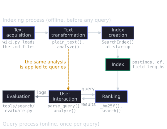
The search box at the top of this site is a complete, small instance of the diagram. When the site starts, app/wiki.py reads the article files (acquisition), app/search.py strips their Markdown and analyzes the text (transformation), and the SearchIndex class builds an inverted index with term positions, stored separately for the title, summary, headings and body of each article (index creation). A query is parsed by app/query.py, analyzed by the same function used on the articles, scored with BM25F, and returned with highlighted snippets. Its evaluation runs offline: a file of about sixty known-item queries, each paired with the article it should find, scores the ranking whenever its parameters are tuned (tools/search/evaluate.py), and the build fails if any article is not the top result for its own title. Because nothing in it is hidden, it can be traced stage by stage, which a later section does.
Why the work is split this way
The split exists because the two processes face different constraints. Indexing can be slow, because it runs in the background, ahead of any query, and can be spread across many machines. Query processing must be fast, because a person is waiting. Anything that does not depend on the query should therefore be computed at indexing time: tokenizing documents, counting terms, computing document lengths and collection statistics, and, on the web, computing link-based authority scores. The query process is left with only the work that genuinely depends on the query.
The principle can be pushed further than it first appears. In BM25 and its relatives, the contribution a term makes to a document's score depends only on the term and the document, not on the other words of the query. It can therefore be computed once, at indexing time, for every term and every document that contains it. This site does exactly that for the instant results that appear as a reader types: the server exports, for each term, the list of articles containing it with each article's precomputed contribution, and the browser answers a query by adding up the numbers for its terms. The browser contains no stemmer and no scoring formula (a typed word is mapped to its index term through an exported word list), yet for any word the wiki uses it ranks exactly as the server does, because every part of the score that could be computed in advance was. The price is flexibility: changing a ranking parameter means recomputing the exported weights.
The split is less clean in practice. A news search engine must make new articles searchable within minutes, so indexing becomes a continuous process that merges small fresh indexes into a large main one. Caches store the results of frequent queries, which in effect precomputes part of the query process. The article on search at scale covers these mechanisms. The conceptual division still holds: work that can be moved before the query arrives should be.
A small collection, end to end
The stages are easiest to understand on a collection small enough to follow by hand. Consider four documents:
| ID | Text |
|---|---|
| d1 | Arctic sea ice is declining as the climate warms. |
| d2 | A warming climate threatens Arctic seabirds and their food. |
| d3 | Climate models predict warmer winters in Europe. |
| d4 | Seabirds of the Arctic: a field guide. |
Acquisition and parsing
In a real system, acquisition is a substantial problem in itself. A crawler must find documents, decide which to fetch and how often to revisit them, and avoid overloading the servers it visits; this is the subject of web crawling. Parsing must then extract clean text from each format. It has to strip HTML markup and scripts and separate a page's main content from its navigation menus. With PDF files, it must reconstruct reading order: a naive extractor reading a two-column scientific paper line by line across the page interleaves sentences from both columns and produces text that matches nothing. Character encodings must be identified correctly, or non-English text is corrupted before it reaches the index. Here the documents are already plain sentences, so parsing is trivial.
Text analysis
Text analysis turns each document into a list of index terms. This example uses three common steps, each covered properly in text processing and indexing:
- Tokenization: lowercase the text and split it into words, discarding punctuation.
- Stop-word removal: drop very frequent function words, here a, and, as, in, is, of, the, their.
- Stemming: reduce each word to a stem with the Porter stemmer (Porter, 1980), so that inflected forms of a word match one another.
The result, computed with the Porter algorithm as originally published:
| ID | Index terms |
|---|---|
| d1 | arctic, sea, ic, declin, climat, warm |
| d2 | warm, climat, threaten, arctic, seabird, food |
| d3 | climat, model, predict, warmer, winter, europ |
| d4 | seabird, arctic, field, guid |
Several features of this output are worth noting, because they recur in every real system. Stems are not words: climate becomes climat, and ice becomes ic. That does no harm, because the same rules are applied to queries and the stem only needs to be consistent, not readable. Warms and warming both become warm, which is the purpose of stemming. But warmer stays warmer, because the Porter rules do not remove -er from so short a stem, so d3 will not match a query about warming. Stemming trades errors in both directions. It fails to join some related words, as here, and it joins some unrelated ones: the Porter stemmer reduces both university and universe to univers.
Index construction
The inverted index maps each term to its postings list: the documents that contain the term, here with the number of occurrences of the term in each (its term frequency, $tf$). The number of documents in a term's postings list is its document frequency, $df$.
| Term | $df$ | Postings (document: $tf$) |
|---|---|---|
| arctic | 3 | d1: 1, d2: 1, d4: 1 |
| climat | 3 | d1: 1, d2: 1, d3: 1 |
| seabird | 2 | d2: 1, d4: 1 |
| warm | 2 | d1: 1, d2: 1 |
| declin, europ, field, food, guid, ic, model, predict, sea, threaten, warmer, winter | 1 each | one document each |
The index is "inverted" because it reverses the natural organization of the collection. A document lists its words; the index lists, for each word, its documents. That reversal lets a query touch only the postings of its own terms rather than every document. For a query of three terms over a web-scale collection, that is the difference between reading three lists and reading billions of documents.
Query processing
Suppose the query is arctic climate warming. The query goes through the same analysis as the documents and becomes arctic, climat, warm. This consistency is essential. If documents were stemmed and queries were not, warming would match nothing, because the index contains only warm. Every normalization that changes the form of index terms, such as case folding or stemming, must be mirrored at query time.
Query processing in real systems does more than this. It may correct spelling, recognize phrases and named entities, expand the query with synonyms, or rewrite it entirely. The article on web search describes these steps.
Retrieval and ranking
The simplest retrieval model is Boolean. The query arctic AND climat AND warm intersects the three postings lists:
$$\{d1, d2, d4\} \cap \{d1, d2, d3\} \cap \{d1, d2\} = \{d1, d2\}.$$
The result is a set, with no order and no partial credit: d3, which is about a warming climate, and d4, which is about the Arctic, are both excluded. Intersecting postings lists covers how such intersections are computed efficiently.
A ranked model scores every document that contains at least one query term. A simple score sums, over the query terms in a document, the term frequency times a weight for the term's rarity:
$$\text{score}(q, d) = \sum_{t \in q \cap d} tf_{t,d} \cdot \log_{10} \frac{N}{df_t},$$
where $N = 4$ is the number of documents. The logarithmic factor is the inverse document frequency (IDF). A term found in every document gets weight $\log_{10} 1 = 0$, because its presence tells the system nothing. For this collection:
| Term | $df$ | IDF $= \log_{10}(4/df)$ |
|---|---|---|
| arctic | 3 | 0.125 |
| climat | 3 | 0.125 |
| warm | 2 | 0.301 |
Each term appears at most once per document, so each score is the sum of the IDF weights of the query terms the document contains:
| Document | Query terms present | Score |
|---|---|---|
| d1 | arctic, climat, warm | 0.125 + 0.125 + 0.301 = 0.551 |
| d2 | arctic, climat, warm | 0.551 |
| d3 | climat | 0.125 |
| d4 | arctic | 0.125 |
The ranking is d1 and d2 tied, then d3 and d4 tied. Even this tiny example shows the main problems of ranking. Warm counts more than arctic because it is rarer in this collection, not because it is more important to the searcher. The ties need breaking: a real system might prefer shorter documents, fresher ones, or more authoritative ones. And d3 is penalized for a stemming decision, not for its content. The vector space model develops this kind of scoring properly, with length normalization and alternative weightings, and BM25 refines it further.
Presentation
The final stage turns the ranking into something a person can use. Each result is shown with a title, a link, and a snippet. The best snippets are query-dependent: rather than showing the first lines of the document, the system selects passages that contain the query terms. For a query such as symptoms of influenza, a snippet listing the symptoms lets the searcher judge the result, or even satisfy the need, without opening the page. Generating snippets requires access to the document text at query time, so search engines keep the text of each document, as a cached copy or in a separate document store, alongside the index.
The same collection in this site's search engine
The walk-through above used a scoring formula simple enough to compute by hand. A working engine differs in its details, and seeing exactly where is the best preparation for the later topics. This section feeds the same four sentences to this site's own search code (app/search.py), each sentence placed in the body field of an otherwise empty article, and records what every stage produces. The numbers come from tools/experiments/foundations/site_engine_trace.py, which builds the index with the site's own classes; scores are rounded to four decimal places.
Analysis
The engine folds accents and case, splits the text into runs of letters and digits, drops the words on a 33-word stop list, and stems the rest with the Porter algorithm. Its stop list is longer than the eight words used above, but for these sentences it removes the same words, so the index terms are identical to the table in Text analysis:
| ID | Tokens (stop words in brackets) | Length |
|---|---|---|
| d1 | arctic sea ice [is] declining [as] [the] climate warms | 9 |
| d2 | [a] warming climate threatens arctic seabirds [and] [their] food | 9 |
| d3 | climate models predict warmer winters [in] europe | 7 |
| d4 | seabirds [of] [the] arctic [a] field guide | 7 |
One detail is easy to miss. The engine removes stop words from the index but still counts their positions, so a document's length is its number of tokens including stop words, and the term climat sits at position 7 of d1, not position 4. Counting positions this way keeps phrase queries correct when a phrase contains a stop word, as phrase queries explains. The average length of the four documents is $(9 + 9 + 7 + 7)/4 = 8$.
Index
The index stores, for each term, each document that contains it and the positions where it occurs, per field. For the query's three terms, with every occurrence in the body field:
| Term | $df$ | Postings (document: positions) |
|---|---|---|
| arctic | 3 | d1: [0], d2: [4], d4: [3] |
| climat | 3 | d1: [7], d2: [2], d3: [0] |
| warm | 2 | d1: [8], d2: [1] |
The term frequencies of the earlier table are the lengths of these position lists. The whole vocabulary is 16 terms, the same 16 as before.
Parsing the query
The query arctic climate warming goes first to the query parser, which recognizes the site's query language: quoted phrases, + and - signs, field prefixes such as title:, and the Boolean operators AND, OR and NOT. This query has none of them, so the parser returns a free-text query, in which any document containing at least one term is a candidate. Analysis then turns the three words into the index terms arctic, climat and warm, by the same function that analyzed the documents. Had the query been typed as arctic AND climate AND warming, the parser would have built a Boolean tree instead, and only d1 and d2, the intersection computed earlier, would have matched.
Scoring
The engine ranks with BM25F, a variant of BM25 for documents with several fields. With only a body field it reduces to BM25 with $k_1 = 1.2$ and $b = 0.5$. Each term contributes
$$\text{IDF}(t) \cdot \frac{tf'}{k_1 + tf'}, \qquad tf' = \frac{tf}{1 - b + b \cdot L_d / \bar L},$$
where $L_d$ is the document's length and $\bar L$ the average length. Three differences from the hand-worked TF-IDF score are visible in this formula, and the trace shows each of them.
A different IDF. The engine uses $\text{IDF}(t) = \ln\left(1 + \frac{N - df_t + 0.5}{df_t + 0.5}\right)$, the form used by Lucene. It never reaches zero, so even a term found in every document counts a little. For arctic and climat, $\ln(1 + 1.5/3.5) = 0.3567$; for warm, $\ln(1 + 2.5/2.5) = \ln 2 = 0.6931$. The rarer term still counts about twice as much.
Length normalization. The divisor $1 - b + b L_d/\bar L$ is $1.0625$ for d1 and d2, which are longer than average, and $0.9375$ for d3 and d4, which are shorter. A single occurrence in a short document is worth slightly more than one in a long document.
Saturation. $tf'/(k_1 + tf')$ grows with term frequency but can never exceed 1, so the tenth occurrence of a word adds far less than the first.
| Document | Divisor | $tf'$ | $tf'/(k_1 + tf')$ | Term contributions | Score |
|---|---|---|---|---|---|
| d1 | 1.0625 | 0.9412 | 0.4396 | arctic 0.1568, climat 0.1568, warm 0.3047 | 0.6182 |
| d2 | 1.0625 | 0.9412 | 0.4396 | arctic 0.1568, climat 0.1568, warm 0.3047 | 0.6182 |
| d3 | 0.9375 | 1.0667 | 0.4706 | climat 0.1678 | 0.1678 |
| d4 | 0.9375 | 1.0667 | 0.4706 | arctic 0.1678 | 0.1678 |
The ranking agrees with the hand computation, d1 and d2 tied above d3 and d4 tied. (The engine breaks exact ties alphabetically by title; these documents have no titles, so they keep their original order.) On this query the refinements change the scores but not the order. On others they change the order. For the one-word query arctic, TF-IDF gives d1, d2 and d4 the same score of 0.125, while BM25F puts d4 first (0.1678 against 0.1568), because d4 is shorter: one occurrence among 7 tokens counts for more than one among 9. Whether that is the right call is exactly the kind of question evaluation exists to answer.
Snippets and spelling
Each result is shown with the sentence that contains the most distinct query terms, with the matching words highlighted. Here every document is a single sentence, so d2's snippet is the whole sentence with warming, climate and Arctic marked: the highlighter stems each word of the sentence and marks those whose stems are query terms, so the query word warming also lights up warms in d1.
The engine also corrects spelling before it gives up on a word. For the query arctic climat warmng, the stem of warmng is not in the index, so the engine looks for an indexed word within a small edit distance and finds warming, one insertion away. climat is a subtler case: it stems to an indexed term, so it would match, but no document ever uses the word as typed, and the engine offers the usual spelling climate. It runs the corrected query arctic climate warming and says so above the results ("Showing results for ..."), the second of the three rewriting policies described in how a web search engine answers a query. Spelling correction covers the methods.
Try it
The demo below runs the same pipeline on the same four documents, for any query. It shows the stop words dropped, the stems, the postings each term retrieves, the Boolean intersection, and the ranking under both the article's TF-IDF score and the site's BM25F. Queries worth trying: warmer winters, which only d3 matches, because the stemmer keeps warmer apart from warm; the seabirds of europe, whose Boolean intersection is empty while the ranked list still has three documents; and arctic, where the two scores disagree. The demo treats every query as free text: it has no query parser, so quotes, signs and the words AND, OR and NOT are not operators here (the last three are stop words and vanish). Its stemmer gives the same stems as the site's on every word the wiki uses, and tools/experiments/foundations/pipeline_trace_check.py compares its scores with the engine's.
At full size
The same code indexes the whole wiki when the site starts. In November 2026, when it held 152 articles and topic pages, the index had roughly 9,600 distinct terms, 97,000 postings (term and article pairs) and 330,000 recorded positions, built from about 460,000 tokens in a second or two. A query such as how a search engine answers a query matched every article, because how occurs in nearly all of them, and was ranked in a few milliseconds on a laptop, with this article's neighbour how a web search engine answers a query first. These figures are a snapshot and move as the wiki grows; the second part of site_engine_trace.py recomputes them for the current wiki. A collection of this size needs none of the machinery of search at scale: one process holds the whole index in memory, and a query touches only a handful of postings lists.
How the stages constrain one another
The pipeline diagram suggests independent stages, each passing its output to the next. In practice each stage limits what the stages after it can do, and the most important limits are set at indexing time.
A ranking function can use only the document information that indexing stored. The scoring above needed term frequencies and document frequencies; an index that recorded only which documents contain each term could support Boolean retrieval but not this ranking. The requirements grow with the model:
| Capability | What the index must store |
|---|---|
| Boolean retrieval | Document IDs in each postings list |
| Vector space ranking | Term frequencies, document frequencies, document lengths or vector norms |
| BM25 | Term frequencies, document frequencies, each document's length, the average document length |
| Phrase and proximity queries | The position of each occurrence of each term |
| Field weighting (title versus body) | Postings separated by field, or field information in each posting |
None of these can be added at query time. If term positions are not stored, then for the phrase query "new york university" a document containing the phrase cannot be distinguished from one that mentions new in one paragraph and York University in another, short of re-reading every candidate document. Adding the capability means rebuilding the index. A positional index is typically two to four times larger than one that records only document IDs and frequencies (Manning, Raghavan, and Schütze, 2008, §2.4), so the decision trades storage and speed for query capability, and it has to be made before the system is in use.
Ranking cannot repair analysis errors. If the stemmer conflates university and universe and the index stores only stems, no ranking function can tell them apart, because the index no longer contains the distinction. If it fails to conflate warmer and warm, no ranking function can recover the match; only a change outside ranking, such as query expansion, can add it back. Choosing stop words has the same character: removing the and who saves space but makes the band The Who unsearchable. These decisions sit at the start of the pipeline and are easy to overlook, but they bound the effectiveness of everything after them.
The query must be analyzed like the documents. Any unintended difference between document and query analysis, such as a different tokenizer, a different stemmer version, or a stop-word list applied to one but not the other, produces silent mismatches. Well-designed systems define one analysis component and use it on both paths, a principle the article on modular design builds into the structure of the code.
Presentation feeds back into ranking. What people click, skip, and reformulate is logged, and those logs become training data for ranking and query suggestion. Relevance feedback makes the loop explicit by asking the searcher to mark relevant results and re-running the query. The pipeline is therefore closer to a cycle: the output of the last stage changes the behavior of the earlier ones over time.
The consequence is that improving a search engine rarely means improving one stage in isolation. An excellent ranking function over an index that lost the relevant distinctions will still rank poorly. A carefully written query will fail if analysis and indexing cannot represent what it asks for.
What the diagram leaves out
The architecture described here is an abstraction, and real systems add a great deal to it. A web search engine distributes its index across thousands of machines and replicates it for capacity, so that a single query is answered by many servers working in parallel. It ranks in several stages, applying a cheap function to many candidates and expensive models to only the best few hundred. It detects spam and near-duplicate pages, personalizes results, and updates its index continuously. Enterprise and domain-specific systems add access control, structured fields, and specialized vocabularies. The web search and scale articles describe these additions, and search applications describes how the architecture is adapted to different settings.
The same underlying structure persists through all of them. Documents become terms, terms become an index, a query becomes terms analyzed the same way, and a ranking function uses the index to order candidates. The rest of the course examines each of those steps.
References
- Croft, W. B., Metzler, D., and Strohman, T. (2010). Search Engines: Information Retrieval in Practice, chapter 2. Addison-Wesley.
- Manning, C. D., Raghavan, P., and Schütze, H. (2008). Introduction to Information Retrieval, chapters 1–2 and 6. Cambridge University Press.
- Porter, M. F. (1980). An algorithm for suffix stripping. Program, 14(3), 130–137.