Take two objectives, both to be minimized, whose best trade-offs lie on the curve $f_2 = 1 - f_1^2$ for $0 \le f_1 \le 1$. The obvious way to handle two objectives is to add them with weights and minimize the sum $w f_1 + (1 - w) f_2$. Trying eleven evenly spaced weights, $w = 0, 0.1, \dots, 1$, gives eleven single-objective problems, and solving each exactly returns exactly two distinct answers: $(f_1, f_2) = (1, 0)$ for every $w < 0.5$, and $(0, 1)$ for every $w > 0.5$. At $w = 0.5$ the two ends tie. No choice of weights, however fine the sweep, reaches any of the trade-offs in between.
Turning a multi-objective problem into one or more single-objective problems is called scalarization. It is the classical approach, much older than multi-objective evolutionary algorithms, and it is still often the right one. Different scalarizations reach different parts of the Pareto-optimal front, and the example above shows the best known failure. This article explains that failure, then two methods that avoid it, then the cases where scalarization is the better tool.
Scalarization
A scalarization replaces the vector of objectives $\mathbf{f} = (f_1, \dots, f_M)$ by a single function $s(\mathbf{f}(\mathbf{x}); \mathbf{p})$ with parameters $\mathbf{p}$, such as weights or bounds, and minimizes it with any single-objective method. One solve yields one point. A representative set of points on the front comes from solving again with different parameters. Miettinen (1999, Part II, ch. 3) calls methods used this way a posteriori methods: the points are generated first and the decision maker chooses among them afterwards. The same scalarizations can also be used a priori, with parameters that encode the decision maker's preferences, to produce a single answer.
Three properties decide whether a scalarization is useful. Its minimizers should be Pareto optimal, or at least weakly Pareto optimal. Every Pareto-optimal point should be the minimizer for some choice of parameters. And the parameters should control where on the front the solution lands, so that evenly spaced parameters give a reasonably even spread of points. The weighted sum has the first property, has the second only for convex problems, and lacks the third.
The weighted sum
The weighted sum method solves
$$\min_{\mathbf{x} \in S} \; \sum_{i=1}^{M} w_i f_i(\mathbf{x}), \qquad w_i \ge 0, \quad \sum_{i=1}^{M} w_i = 1.$$
Its basic results (Miettinen, 1999, Part II, §3.1): a minimizer is weakly Pareto optimal whenever the weights are nonnegative, and Pareto optimal if all weights are positive or if the minimizer is unique. Conversely, if the problem is convex (convex objectives on a convex feasible set), every Pareto-optimal point minimizes the weighted sum for some nonnegative weights.
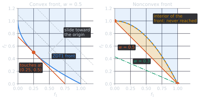
The geometry explains both results. In objective space, with two objectives, the points of equal weighted sum $w_1 f_1 + w_2 f_2 = c$ form a straight line with slope $-w_1 / w_2$. Minimizing the sum means sliding that line toward the origin, keeping its slope, until it last touches the attainable set $Z$. The touching point is the solution. The weights fix only the direction of the line. A point is reachable exactly when some line touches $Z$ there and has all of $Z$ on one side.
Two worked cases show the picture in numbers. Take $w = 0.5$, so the lines have slope $-1$.
- On the convex front $f_2 = 1 - \sqrt{f_1}$, the sum along the front is $0.5 f_1 + 0.5 (1 - \sqrt{f_1})$. Its derivative with respect to $f_1$ is $0.5 - 0.25 / \sqrt{f_1}$, which is zero at $\sqrt{f_1} = 0.5$. The minimizer is $(f_1, f_2) = (0.25, 0.5)$ and the minimum is $0.375$. The line $0.5 f_1 + 0.5 f_2 = 0.375$ touches the front there and nowhere else, and lies below it everywhere else, since the front is convex.
- On the nonconvex front $f_2 = 1 - f_1^2$, the sum along the front is $0.5 f_1 + 0.5 (1 - f_1^2)$. Its second derivative is $-1$, so it is a concave function of $f_1$ and has no interior minimum: its smallest value on $[0, 1]$ is at an end. Both ends give $0.5$, and the midpoint $f_1 = 0.5$ gives $0.625$, which is worse. The line $0.5 f_1 + 0.5 f_2 = 0.5$ is the chord from $(0, 1)$ to $(1, 0)$. The same holds for every $w$: the second derivative of $w f_1 + (1 - w)(1 - f_1^2)$ is $-2(1 - w) \le 0$, so only the ends can win. At $w = 0.3$ the end values are $0.70$ at $f_1 = 0$ and $0.30$ at $f_1 = 1$, and $(1, 0)$ wins outright.
Why only the convex hull is reachable
The convex hull of the front is the smallest convex set containing it. A front point is reachable when it lies on the lower-left boundary of that hull, the part facing the ideal point, where a supporting line of the kind just described can touch it. Points of a concave stretch of the front, such as the curve in the opening example, lie on the far side of the hull, behind the chord that joins the ends of the stretch. They cannot be reached.
A proof sketch, for two objectives. Let $\mathbf{p}$ be a point on the front, and suppose there are attainable points $\mathbf{a}$ and $\mathbf{b}$ and a $\lambda \in (0, 1)$ such that the point $\mathbf{q} = \lambda \mathbf{a} + (1 - \lambda)\mathbf{b}$ on the segment between them lies below and to the left of $\mathbf{p}$: $q_1 < p_1$ and $q_2 < p_2$. The point $\mathbf{q}$ need not be attainable. For any weights $w_1, w_2 \ge 0$, not both zero, the weighted sum is linear, so
$$\mathbf{w} \cdot \mathbf{p} > \mathbf{w} \cdot \mathbf{q} = \lambda\, \mathbf{w} \cdot \mathbf{a} + (1 - \lambda)\, \mathbf{w} \cdot \mathbf{b} \ge \min(\mathbf{w} \cdot \mathbf{a}, \mathbf{w} \cdot \mathbf{b}).$$
Either $\mathbf{a}$ or $\mathbf{b}$ has a smaller weighted sum than $\mathbf{p}$, whatever the weights, so $\mathbf{p}$ is never the minimizer. On the curve $f_2 = 1 - f_1^2$, every interior point lies strictly above and to the right of the chord from $(0, 1)$ to $(1, 0)$, so the argument applies to all of them with $\mathbf{a} = (0, 1)$ and $\mathbf{b} = (1, 0)$. Conversely, a point on the lower-left boundary of the convex hull has a supporting line, and the slope of that line gives the weights that reach it. Das and Dennis (1997) gave the geometric argument for why weighted sums succeed in reaching all parts of the front only when it is convex, and examined the mechanism behind the uneven spread described next.
The failure is not a defect of a particular optimizer. An exact solver finds the right answer to the weighted-sum problem every time. The question it answers is the wrong one for a nonconvex front. The same effect appears inside evolutionary algorithms that aggregate objectives with weights. Zitzler, Deb, and Thiele (2000) found that on their nonconvex test function, three algorithms based on weighted aggregation or on separate objectives had difficulty finding intermediate solutions, and attributed this to linear combinations of objectives preferring solutions that are strong in at least one objective.
Uneven spread under even weights
Even on a convex front, evenly spaced weights do not give evenly spaced points (Das and Dennis, 1997). The reason is that a weight vector selects a slope, and the front's slope changes at different rates in different places. Where the front bends sharply, a wide range of slopes is concentrated in a small region, and many weights land there; where it is nearly straight, a small range of slopes covers a long stretch, and few weights land there.
The front $f_2 = 1 - \sqrt{f_1}$ shows this exactly. Setting the derivative of $w f_1 + (1 - w)(1 - \sqrt{f_1})$ to zero gives
$$f_1 = \left(\frac{1 - w}{2w}\right)^2,$$
clipped to $f_1 = 1$ when this exceeds 1, which happens for every $w \le 1/3$. With 101 weights $w = 0, 0.01, \dots, 1$, the script below finds that 34 weights land on the single endpoint $f_1 = 1$, 8 land in $0.5 \le f_1 < 1$, 20 in $0.1 \le f_1 < 0.5$, and 39 in $0 \le f_1 < 0.1$. Half the range of $f_1$ receives 8 distinct solutions; the first tenth receives 39. Rescaling the objectives changes which weights land where but does not remove the effect, since any rescaling of a curved front still has slopes concentrated somewhere. Das and Dennis (1998) later proposed normal-boundary intersection, which spaces points evenly on the convex hull of the single-objective optima and intersects the front with lines normal to that hull, to obtain an even spread.
Units decide what a weight means
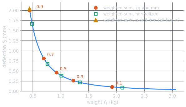
A weight multiplies a quantity measured in some unit, so the same weight means different things in different units. The cantilever beam shows this. Its front is $f_2 = K / f_1^2$ with $K = 0.3940$, weight $f_1$ in kilograms between 0.4394 and 3.0631, and deflection $f_2$ in millimetres. Minimizing $w f_1 + (1 - w) K / f_1^2$, the derivative $w - 2(1 - w) K / f_1^3$ vanishes at
$$f_1 = \left( \frac{2 (1 - w) K}{w} \right)^{1/3},$$
clipped to the front's range. Measuring weight in grams multiplies $f_1$ by 1000 inside the sum, which divides the expression in the brackets by 1000. Normalizing each objective by its range on the front, as described in Pareto dominance, multiplies the expression in the brackets by the ratio of the weight range to the deflection range, $2.6237 / 1.9989 = 1.3126$. The script tools/experiments/evolution/scalarization_beam.py evaluates the closed form and confirms each value by direct search over 2,000,001 evenly spaced beam weights $f_1$ along the front. Whatever units the sum uses, the table reports the chosen beam in kilograms and millimetres, rounded to four decimals:
| $w$ | kg and mm: weight, deflection | normalized: weight, deflection | g and mm: weight |
|---|---|---|---|
| 0.1 | 1.9212, 0.1067 | 2.1035, 0.0890 | 0.4394 |
| 0.3 | 1.2251, 0.2625 | 1.3413, 0.2190 | 0.4394 |
| 0.5 | 0.9236, 0.4618 | 1.0113, 0.3852 | 0.4394 |
| 0.7 | 0.6964, 0.8124 | 0.7625, 0.6777 | 0.4394 |
| 0.9 | 0.4440, 1.9981 | 0.4862, 1.6668 | 0.4394 |
Kilograms and normalized units give similar answers here, because the two objectives happen to have ranges of similar size. In grams, the weight term swamps the deflection term, and every $w$ from 0.0092 upward returns the lightest beam. Nothing about the beam changed; only the unit did. Normalizing before weighting removes the dependence on units, but the weights still express a trade-off between normalized quantities, which a decision maker has to interpret.
The ε-constraint method
The ε-constraint method, usually credited to Haimes, Lasdon, and Wismer (1971), keeps one objective and turns the others into constraints:
$$\min_{\mathbf{x} \in S} \; f_\ell(\mathbf{x}) \quad \text{subject to} \quad f_j(\mathbf{x}) \le \varepsilon_j \text{ for all } j \ne \ell.$$
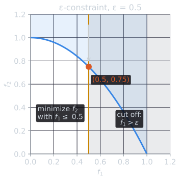
Its results (Miettinen, 1999, Part II, §3.2): every minimizer is weakly Pareto optimal, and a unique minimizer is Pareto optimal. A point $\mathbf{x}^*$ is Pareto optimal if and only if it solves the ε-constraint problem for every choice of $\ell$, with $\varepsilon_j = f_j(\mathbf{x}^*)$. In particular, every Pareto-optimal point can be found, whether or not the problem is convex. Geometrically, the constraint cuts off the part of objective space beyond $\varepsilon$, and the minimizer is the best remaining point in the kept objective. Nothing in that operation depends on the front's curvature.
On the nonconvex front $f_2 = 1 - f_1^2$, keeping $f_2$ and bounding $f_1 \le 0.5$ asks for the lowest $f_2$ among points with $f_1$ at most 0.5. Since $f_2$ falls as $f_1$ rises along the front, the answer sits on the bound: $(0.5, 0.75)$, a point in the middle of the stretch that no weighted sum can reach.
The constraint form is also how engineers often state the problem in the first place. For the cantilever beam, "the lightest beam that deflects at most $\varepsilon$" keeps weight as the objective and bounds deflection. On the front $f_2 = 0.3940 / f_1^2$, the bound is active at the optimum, so the answer is $f_1 = \sqrt{0.3940 / \varepsilon}$, and the diameter at $l = 200$ mm follows from the weight. From scalarization_beam.py:
| ε (mm) | Weight (kg) | Diameter (mm) |
|---|---|---|
| 2.00 | 0.4438 | 19.03 |
| 1.00 | 0.6277 | 22.63 |
| 0.50 | 0.8877 | 26.92 |
| 0.25 | 1.2553 | 32.01 |
| 0.10 | 1.9849 | 40.25 |
| 0.05 | 2.8070 | 47.86 |
Halving the allowed deflection multiplies the weight by $\sqrt{2} = 1.414$ each time, which the table shows from 2 mm down to 0.25 mm. A bound of 2.0409 mm or more, the nadir deflection, returns the lightest feasible beam, and a bound below 0.0420 mm, the ideal deflection, has no feasible solution.
The method has its own costs. The bounds must be chosen within the range of the front, between the ideal and nadir values: a bound below the ideal value makes the problem infeasible, and one above the nadir value has no effect. With $M$ objectives, a grid of $k$ values per constrained objective needs $k^{M-1}$ solves, many of them infeasible or redundant. The added constraints make each subproblem harder for some solvers than an unconstrained one. And even spacing of $\varepsilon$ gives even spacing in the constrained objective, not along the front, so steep parts of the front are sampled sparsely.
Tchebycheff and achievement scalarizing functions
A third family measures distance to a reference point rather than a weighted total. The weighted Tchebycheff problem minimizes the largest weighted deviation from a utopian point $\mathbf{z}^{**}$, slightly better than the ideal point in every objective:
$$\min_{\mathbf{x} \in S} \; \max_{i = 1, \dots, M} \; w_i \big(f_i(\mathbf{x}) - z_i^{**}\big).$$
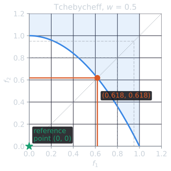
Its level sets are the corners of boxes centered on the reference point, not straight lines, so they can reach into a concave stretch of the front. Every Pareto-optimal point is a solution for some positive weights, convex or not, but a solution may be only weakly Pareto optimal (Miettinen, 1999, Part II, §3.4). Adding a small term $\rho \sum_i (f_i - z_i^{**})$, with $\rho > 0$, gives the augmented Tchebycheff problem, whose solutions are Pareto optimal; the price is that, for a given $\rho$, Pareto-optimal points where the trade-off rate between objectives is very large may no longer be reachable (Miettinen, 1999, Part II, §3.4).
The equal-weight case can be solved by hand. With $w_1 = w_2 = 0.5$ and the reference point at the ideal point $(0, 0)$, as in the sweep below, the problem is to minimize $0.5 \max(f_1, f_2)$ along the front. Moving along the front, $f_1$ rises while $f_2$ falls, so the larger of the two is smallest where they are equal: the solution lies where the front crosses the diagonal $f_1 = f_2$. On $f_2 = 1 - f_1^2$, setting $f_1 = 1 - f_1^2$ gives $f_1^2 + f_1 - 1 = 0$, whose positive root is $f_1 = (\sqrt{5} - 1)/2 = 0.6180$. On $f_2 = 1 - \sqrt{f_1}$, substituting $t = \sqrt{f_1}$ gives $t^2 + t - 1 = 0$, the same equation, so $t = 0.6180$ and $f_1 = t^2 = 0.3820$. Other weights tilt the diagonal: the corner of the level set moves along the ray $w_1 f_1 = w_2 f_2$, and on a connected front such as these the solution is where that ray meets the front, whatever the front's curvature.
Wierzbicki (1980) generalized this into achievement scalarizing functions. The decision maker supplies a reference point $\mathbf{q}$ of aspiration levels, the objective values he or she would like to reach, and the method minimizes a function such as
$$s(\mathbf{f}; \mathbf{q}) = \max_{i} \, w_i (f_i - q_i) + \rho \sum_i w_i (f_i - q_i).$$
The reference point may be attainable or not. If it is unattainable, the minimizer is a Pareto-optimal point that comes as close to the aspirations as the problem allows; if it is attainable, the minimizer is at least as good as it in every objective. Moving the reference point moves the solution in a predictable way, which is why these functions underlie many interactive methods (Miettinen, 1999, Part II, §3.5).
The sweep on ZDT1 and ZDT2
Zitzler, Deb, and Thiele (2000) defined six two-objective test functions, $T_1$ to $T_6$, now known as ZDT1 to ZDT6. The first two have $m = 30$ variables in $[0, 1]$ and share a structure:
$$f_1 = x_1, \qquad g = 1 + \frac{9}{m - 1} \sum_{i=2}^{m} x_i, \qquad f_2 = g \cdot h(f_1, g),$$
with $h = 1 - \sqrt{f_1 / g}$ for ZDT1 and $h = 1 - (f_1/g)^2$ for ZDT2. The Pareto-optimal set is $x_2 = \dots = x_m = 0$, where $g = 1$, so the fronts are $f_2 = 1 - \sqrt{f_1}$ (convex) and $f_2 = 1 - f_1^2$ (nonconvex), the curves used above. They are mirror images of each other under the reflection $(f_1, f_2) \mapsto (1 - f_2, 1 - f_1)$, and both have arc length 1.4789. For each fixed $x_1$, $f_2$ increases with $g$, so every scalarized problem here is minimized with $g = 1$, and each reduces to a one-variable problem in $x_1$.
The script tools/experiments/evolution/scalarization.py in the site repository solves each scalarized problem by evaluating it at 1,000,001 evenly spaced values of $x_1$ and taking the minimizer. It runs each method with eleven parameter values $k/10$, $k = 0, \dots, 10$: weights $w$ for the weighted sum $w f_1 + (1-w) f_2$; bounds $\varepsilon$ for minimizing $f_2$ subject to $f_1 \le \varepsilon$; and weights $w$ for the augmented Tchebycheff function $\max(w f_1, (1 - w) f_2) + 10^{-4}(f_1 + f_2)$ with reference point $(0, 0)$, the ideal point. "Largest gap" is the longest stretch of the front, as a percentage of its arc length, between consecutive distinct solutions or between a solution and an end of the front.
| Method | ZDT1 distinct points | ZDT1 largest gap | ZDT2 distinct points | ZDT2 largest gap |
|---|---|---|---|---|
| Weighted sum | 8 | 34.1% | 2 | 100.0% |
| ε-constraint | 11 | 22.7% | 11 | 14.5% |
| Augmented Tchebycheff | 11 | 20.1% | 11 | 12.0% |
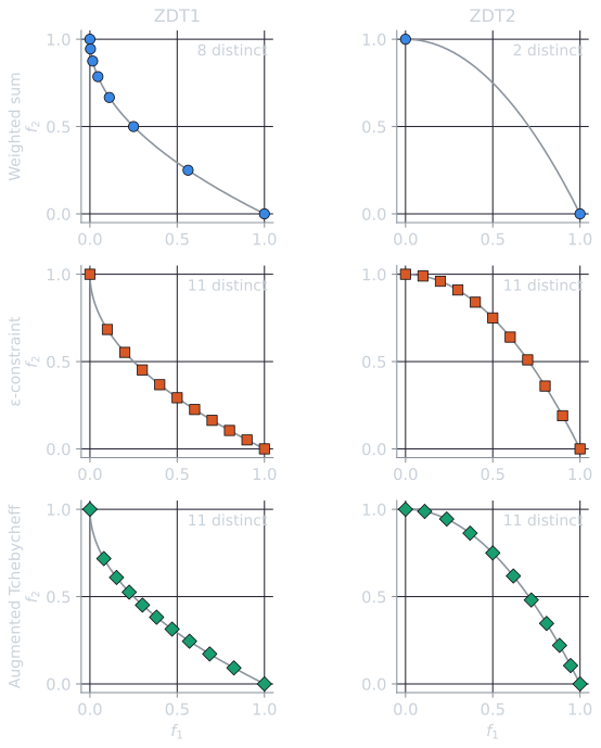
On the convex front, the weighted sum reaches eight distinct points: four weights ($w \le 0.3$) all give the endpoint $(1, 0)$, and the others give $f_1$ = 0.5625, 0.25, 0.1111, 0.0459, 0.0156, 0.0031 and 0, crowding toward $f_1 = 0$. On the nonconvex front it reaches only the two endpoints, so the gap between them is the whole front. The ε-constraint method reaches $f_1 = \varepsilon$ exactly on both problems, which is even in $f_1$ but leaves its largest gap where the front is steepest: near $f_1 = 0$ on ZDT1, where $f_2$ falls from 1 to 0.6838 between the first two points, and near $f_1 = 1$ on ZDT2. The Tchebycheff weights give the most even spread of the three on both fronts. With equal weights its solution is the point where $f_1 = f_2$: 0.3820 on ZDT1 and 0.6180 on ZDT2, which are $1/\varphi^2$ and $1/\varphi$ for the golden ratio $\varphi$, and which the mirror symmetry maps onto each other.
When scalarization beats an evolutionary algorithm
An evolutionary multi-objective algorithm such as NSGA-II approximates the whole front in one run, without assumptions about its shape. Scalarization finds one point per solve, but each solve can use any single-objective method, including gradient-based methods with fast convergence and optimality conditions that certify the result. The comparison favors scalarization in several situations.
- The preferences are known. If the decision maker can state weights, bounds or a reference point before the search, one scalarized solve answers the question. Approximating the whole front only to discard most of it wastes evaluations.
- The problem is smooth and well behaved. For differentiable objectives and constraints, a gradient-based solver typically reaches each Pareto-optimal point to high accuracy in few evaluations, and a convex problem has no local fronts to trap it. An evolutionary algorithm converges to the front only approximately and gives no certificate that it has arrived.
- Only a few points are needed. With two or three objectives, a handful of ε-constraint or Tchebycheff solves may describe the front well enough, especially with an exact solver, while a population-based method must evaluate many solutions to make its front converge.
The evolutionary approach has the advantage in the opposite cases: black-box or multimodal objectives where single-objective solvers also stall in local optima, fronts that are nonconvex or disconnected, many points wanted at once, or preferences that are unclear until the trade-offs are seen (Deb, 2001; Eiben and Smith, 2015, ch. 12). The two approaches also combine. MOEA/D (Zhang and Li, 2007) decomposes a multi-objective problem into many scalar subproblems, using weighted sums, Tchebycheff functions or a boundary-intersection method, and optimizes them simultaneously in one population, each subproblem drawing on information from its neighbors. A common practical pattern runs an evolutionary algorithm first to see the shape of the front, then refines chosen points with a scalarized local solver.
References
- Das, I., and Dennis, J. E. (1997). A closer look at drawbacks of minimizing weighted sums of objectives for Pareto set generation in multicriteria optimization problems. Structural Optimization, 14(1), 63–69.
- Das, I., and Dennis, J. E. (1998). Normal-boundary intersection: A new method for generating the Pareto surface in nonlinear multicriteria optimization problems. SIAM Journal on Optimization, 8(3), 631–657.
- Deb, K. (2001). Multi-Objective Optimization Using Evolutionary Algorithms. John Wiley & Sons.
- Eiben, A. E., and Smith, J. E. (2015). Introduction to Evolutionary Computing, 2nd ed., chapter 12. Springer.
- Haimes, Y. Y., Lasdon, L. S., and Wismer, D. A. (1971). On a bicriterion formulation of the problems of integrated system identification and system optimization. IEEE Transactions on Systems, Man, and Cybernetics, SMC-1(3), 296–297.
- Miettinen, K. (1999). Nonlinear Multiobjective Optimization. Kluwer Academic Publishers.
- Wierzbicki, A. P. (1980). The use of reference objectives in multiobjective optimization. In G. Fandel and T. Gal (Eds.), Multiple Criteria Decision Making Theory and Application, 468–486. Springer.
- Zhang, Q., and Li, H. (2007). MOEA/D: A multiobjective evolutionary algorithm based on decomposition. IEEE Transactions on Evolutionary Computation, 11(6), 712–731.
- Zitzler, E., Deb, K., and Thiele, L. (2000). Comparison of multiobjective evolutionary algorithms: Empirical results. Evolutionary Computation, 8(2), 173–195.