Nine candidate designs have been evaluated on two objectives to be minimized, say cost and weight:
| Design | A | B | C | D | E | F | G | H | I |
|---|---|---|---|---|---|---|---|---|---|
| $(f_1, f_2)$ | (1, 8) | (2, 5) | (4, 4) | (6, 2) | (9, 1) | (3, 7) | (5, 5) | (7, 3) | (8, 6) |
Only seven may survive into the next generation. Which seven? A single-objective algorithm would sort by fitness and keep the top seven, but here no single order exists. B is better than F in both objectives, so F should rank below B, but A and E are each best in one objective and cannot be compared at all. A multi-objective genetic algorithm has to answer two questions to make the choice: which designs are closest to the Pareto front, and among designs that are equally close, which ones keep the population spread along it.
NSGA-II (Deb, Pratap, Agarwal and Meyarivan, 2002) answers the first question with non-dominated sorting and the second with a crowding distance, and it keeps the best designs found so far by choosing survivors from parents and offspring together. It became one of the most widely used multi-objective evolutionary algorithms. This article specifies it fully, works through the example above, and reports a seeded reproduction of its experiments on three standard test problems.
Why a second version
Its predecessor, NSGA (Srinivas and Deb, 1994), sorted the population into fronts of mutually non-dominated individuals and used fitness sharing to spread each front. Deb et al. (2002) list three criticisms that it had attracted:
- Cost. Its sorting procedure needed $O(MN^3)$ operations per generation for $M$ objectives and population size $N$.
- No elitism. A Pareto-optimal solution, once found, could be lost in the next generation. Zitzler, Deb and Thiele (2000) had found elitism to be an important factor in multi-objective search.
- A sharing parameter. Fitness sharing needs a niche radius $\sigma_{\text{share}}$ (see selection pressure and premature convergence), and the spread it achieves depends heavily on that choice.
NSGA-II replaces the sorting procedure, adds survivor selection from parents and offspring combined, and replaces sharing with a parameter-free density estimate.
Fast non-dominated sorting
Solution $p$ dominates $q$ if $p$ is no worse than $q$ in every objective and strictly better in at least one. The first front $\mathcal{F}_1$ is the set of solutions that nothing dominates; the second front is what is non-dominated once $\mathcal{F}_1$ is removed, and so on. Rank is the index of a solution's front.
A naive procedure finds each front by comparing every remaining pair, $O(MN^2)$ per front, and with up to $N$ fronts it costs $O(MN^3)$. The fast procedure compares each pair only once. For every solution $p$ it records two things:
- $n_p$, the domination count: the number of solutions that dominate $p$;
- $S_p$, the set of solutions that $p$ dominates.
Then:
- Compare every pair of solutions, filling in all $n_p$ and $S_p$.
- Put every solution with $n_p = 0$ in $\mathcal{F}_1$. Set $i = 1$.
- While $\mathcal{F}_i$ is not empty: for each $p \in \mathcal{F}_i$ and each $q \in S_p$, decrease $n_q$ by one, and if $n_q$ reaches 0, put $q$ in $\mathcal{F}_{i+1}$. Then increase $i$.
Step 1 makes $N(N-1)/2$ comparisons of $M$ objectives each, $O(MN^2)$. In step 3 each solution enters exactly one front and its set $S_p$ is traversed once, and each $S_p$ has at most $N - 1$ members, so step 3 costs $O(N^2)$. The total is $O(MN^2)$. The price is memory: the sets $S_p$ take $O(N^2)$ space, where the naive procedure needs $O(N)$ (Deb et al., 2002, §III-A).
In the example, the counts are $n = 0$ for A to E, $n_F = 1$ (dominated by B), $n_G = 2$ (B and C), $n_H = 1$ (D) and $n_I = 5$ (B, C, D, G and H). B dominates F, G and I; C dominates G and I; D dominates H and I; G and H each dominate I. The first front is {A, B, C, D, E}. Processing it, B lowers $n_F$ to 0 and C lowers $n_G$ to 0, and D lowers $n_H$ to 0, so the second front is {F, G, H}. Processing that, G and H lower $n_I$ from 2 to 0, and the third front is {I}.
The whole procedure fits in one table. The columns $n$ and $S$ are the result of step 1; the next two columns show each count after the members of a front have been processed, with a dash once the point has been placed:
| Point | $(f_1, f_2)$ | $n_p$ | $S_p$ | $n$ after front 1 | $n$ after front 2 | Front |
|---|---|---|---|---|---|---|
| A | (1, 8) | 0 | none | – | – | 1 |
| B | (2, 5) | 0 | F, G, I | – | – | 1 |
| C | (4, 4) | 0 | G, I | – | – | 1 |
| D | (6, 2) | 0 | H, I | – | – | 1 |
| E | (9, 1) | 0 | none | – | – | 1 |
| F | (3, 7) | 1 | none | 0 | – | 2 |
| G | (5, 5) | 2 | I | 0 | – | 2 |
| H | (7, 3) | 1 | I | 0 | – | 2 |
| I | (8, 6) | 5 | none | 2 | 0 | 3 |
Two checks are worth making when tracing the procedure by hand. The column $n_p$ sums to the total length of the sets $S_p$, here 9, since each domination relation is counted once from each end. And every count reaches zero exactly when the last of the point's dominators has been placed, so a point's front is one more than the largest front among its dominators: I's dominators lie on fronts 1 and 2, so I lies on front 3. That rule is a useful definition of rank in its own right, and it shows why the fronts are layers. A point on front $k$ is dominated by some point on front $k - 1$, but never by a point on front $k$ or later.
Crowding distance
Within a front, NSGA-II prefers solutions in sparsely populated regions. It estimates density by the crowding distance, roughly the perimeter of the box whose corners are a solution's two neighbours along the front (Deb et al., 2002, §III-B). For a front $\mathcal{I}$ of $l$ solutions:
- Set every distance to 0.
- For each objective $m$: sort $\mathcal{I}$ by $f_m$. Give the first and last solutions, the boundary points, distance $\infty$. For each solution $k = 2, \dots, l-1$ in sorted order, add $$\frac{f_m(k+1) - f_m(k-1)}{f_m^{\max} - f_m^{\min}},$$ where $f_m^{\max}$ and $f_m^{\min}$ are the largest and smallest values of objective $m$.
The normalization by each objective's range makes objectives of different scales comparable, so that cost in dollars does not swamp weight in kilograms. The paper calls $f_m^{\max}$ and $f_m^{\min}$ the maximum and minimum values of the objective; the implementation published by Deb's laboratory takes them over the front being measured, and so does the experiment below. The infinite distance of the boundary points means that the extremes of every front are always preferred, which keeps the population stretched across the whole range of each objective. Each of the $M$ sorts costs $O(N \log N)$, so the procedure is $O(MN \log N)$.
In the example, the first front spans 8 units of $f_1$ (1 to 9) and 7 units of $f_2$ (1 to 8). A and E are boundary points with infinite distance. B lies between A and C in $f_1$ and between C and A in $f_2$:
$$d_B = \frac{4 - 1}{8} + \frac{8 - 4}{7} = 0.375 + 0.5714 = 0.9464.$$
Likewise $d_C = 4/8 + 3/7 = 0.9286$ and $d_D = 5/8 + 3/7 = 1.0536$. In the second front, which spans 4 units in each objective, F and H are boundary points, and $d_G = 4/4 + 4/4 = 2$.
The crowded-comparison operator
With a rank and a crowding distance for every solution, the crowded-comparison operator $\prec_n$ defines which of two solutions is better:
$$i \prec_n j \quad \text{if} \quad r_i < r_j \quad \text{or} \quad (r_i = r_j \text{ and } d_i > d_j),$$
where $r$ is the rank and $d$ the crowding distance. A lower rank wins; within a rank, the less crowded solution wins. The operator is used twice in every generation: in the binary tournaments that choose parents, and in choosing which members of the last admitted front survive.
The main loop
The algorithm starts from a random population $P_0$ of size $N$, sorted into fronts, and creates offspring $Q_0$ of size $N$ by binary tournament selection, crossover and mutation. Each later generation $t$ does the following (Deb et al., 2002, §III-C):
- Combine. Form $R_t = P_t \cup Q_t$, of size $2N$.
- Sort. Sort $R_t$ into fronts $\mathcal{F}_1, \mathcal{F}_2, \dots$
- Fill. Start with an empty $P_{t+1}$. While $\lvert P_{t+1} \rvert + \lvert \mathcal{F}_i \rvert \le N$, compute the crowding distances in $\mathcal{F}_i$, add all of $\mathcal{F}_i$ to $P_{t+1}$, and move on to $\mathcal{F}_{i+1}$.
- Truncate the last front. The first front that does not fit, $\mathcal{F}_l$, is sorted by $\prec_n$ (in practice, by decreasing crowding distance, since its members share a rank), and its first $N - \lvert P_{t+1} \rvert$ members complete $P_{t+1}$.
- Reproduce. Create $Q_{t+1}$ of size $N$ from $P_{t+1}$ by binary tournaments decided by $\prec_n$, followed by crossover and mutation.
The published pseudocode prints the loop condition in step 3 as "until $\lvert P_{t+1} \rvert + \lvert \mathcal{F}_i \rvert \le N$", but the accompanying text makes clear that fronts are admitted for as long as the condition holds, which is how the step is written here. Because parents compete with their offspring, a solution that is non-dominated in $R_t$ can only leave the population if at least $N$ other members of $R_t$ are also non-dominated, which is the elitism that NSGA had lacked. Sorting dominates the cost of a generation, $O(M(2N)^2) = O(MN^2)$. The sorting can stop as soon as the admitted fronts hold $N$ members.
This elitism is weaker than it may sound. It guarantees that a non-dominated solution is never displaced by a dominated one, but when the first front alone holds more than $N$ members, crowding removes some non-dominated solutions, and nothing remembers them. Suppose the nine designs of the example were reduced to $N = 4$: C, the most crowded member of the first front, is discarded, and A, B, D and E survive. If a later offspring lands at $(4.5, 4.5)$, none of A, B, D or E dominates it, so it can enter the population, although C, which the algorithm once held, dominates it. The population has accepted a solution worse than one it had already found. With a fixed population size this cannot be ruled out, since some non-dominated solutions must be forgotten, and the bounded archives of algorithms such as SPEA2, described in multi-objective evolutionary algorithms, face the same problem whenever they are truncated.
For the example with $N = 7$, the first front's five members fit ($5 \le 7$). The second front does not ($5 + 3 > 7$), so it is truncated to two members by crowding distance: F and H, with infinite distance, beat G, with 2. The survivors are A, B, C, D, E, F and H. G is rejected although neither F nor H dominates it, because it lies between the two solutions that hold the front's extremes. The script tools/experiments/evolution/nsga2.py in the site repository prints all of these counts, fronts and distances.
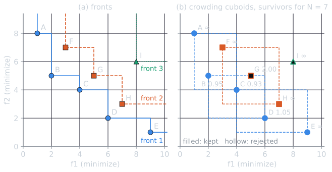
The demo below runs the same procedure step by step. It starts from the nine designs; drag any point, or select it and use the arrow keys, to see how the counts, fronts, distances and survivors change, and move the slider to change $N$.
Two experiments are worth trying. First, with the original points, lower $N$ to 4 and then 3. The first front no longer fits, and its members leave in order of crowding distance: C (0.9286) goes first, then B (0.9464), and the extremes A and E are never removed while an interior point remains. Second, reset and drag G to $(5, 3)$. G is now non-dominated and joins the first front, which grows to six members, and H, now dominated by G as well as D, stays on the second front with F. G's arrival also changes its neighbours' distances: C falls to 0.6607 and D to 0.7857, and G itself, squeezed between C and D, has the smallest, 0.5357. With $N = 7$, G survives with the whole first front. With $N = 5$, it is the first to go. A design that was rejected for being dominated is, after the move, rejected for being crowded. (F and H, both boundary points of the second front, tie at infinite distance; the demo, like the script, keeps whichever comes first in the front, a detail the paper leaves open.)
One generation on ZDT1, traced
The example above is a hand-made set of nine points. In a real run the merged population $R_t$ holds $2N$ members, half of them parents and half their offspring. The script tools/experiments/evolution/nsga2_trace.py follows the first survivor selection of a small run: ZDT1 (defined below) with $n = 30$ variables, $N = 10$, the reference operators, and seed 0. The ten random parents $P_0$ and their ten offspring $Q_0$ form $R_0$, which sorts into fronts of 7, 6, 4 and 3 members. The first front fits, leaving three places for the six members of the second front, which are ranked by crowding distance within that front:
| Member | Origin | $(f_1, f_2)$ | Crowding distance | Kept |
|---|---|---|---|---|
| f | parent | (0.010, 5.960) | $\infty$ | yes |
| r | offspring | (0.927, 3.124) | $\infty$ | yes |
| c | parent | (0.405, 4.563) | 1.009 | yes |
| s | offspring | (0.688, 3.487) | 0.938 | no |
| m | offspring | (0.177, 4.769) | 0.923 | no |
| g | parent | (0.861, 3.312) | 0.388 | no |
Values are rounded to three decimals. The two extremes survive as always, and c, which sits in the widest gap of the front, takes the last place. The new population $P_1$ holds six parents and four offspring; three of the offspring entered on the first front.
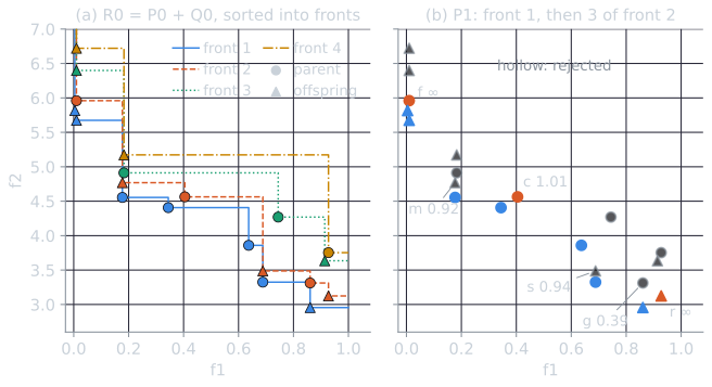
Several offspring share their $f_1$ value exactly with a parent, m with h for example. In ZDT problems $f_1 = x_1$, and a child keeps its parent's $x_1$ unless that variable is crossed, which happens with probability $0.9 \times 0.5$, or mutated, with probability $1/30$. Such a child differs from its parent only in $f_2$, and so it either dominates the parent or is dominated by it, which is why parents and offspring so often land on adjacent fronts at the same $f_1$, as on the left of the figure.
Constrained domination
To handle constraints, Deb et al. (2002, §VI) modify only the definition of domination. Solution $i$ constrained-dominates $j$ if any of the following holds:
- $i$ is feasible and $j$ is not;
- both are infeasible, and $i$ has the smaller overall constraint violation;
- both are feasible, and $i$ dominates $j$ in the usual sense.
Every feasible solution then ranks above every infeasible one, and infeasible solutions are ranked by violation alone. The rest of the algorithm is unchanged, and so is its complexity. The rule is the multi-objective form of Deb's feasibility rules for single-objective problems, described with their strengths and weaknesses in constraint handling in evolutionary algorithms. The paper tested it on four constrained problems, one with five objectives and seven constraints, using a population of 100, 500 generations, and distribution indices of 20 for crossover and 100 for mutation.
Operators and settings in the paper
NSGA-II prescribes selection, not variation. The paper ran a binary-coded version, with 30 bits per variable, single-point crossover and bitwise mutation, and a real-coded version with simulated binary crossover (SBX; Deb and Agrawal, 1995) and polynomial mutation. Both operators draw children near their parents from a polynomial distribution whose spread is set by a distribution index $\eta$, as described in crossover and mutation operators. The settings were (Deb et al., 2002, §IV-A):
| Setting | Value |
|---|---|
| Population size $N$ | 100 |
| Generations | 250 (25,000 function evaluations) |
| Crossover probability $p_c$ | 0.9 |
| Mutation probability $p_m$ | $1/n$ for $n$ real variables, $1/\ell$ for a string of $\ell$ bits |
| SBX distribution index $\eta_c$ | 20 |
| Mutation distribution index $\eta_m$ | 20 |
The authors chose "a reasonable set of values" without tuning. They compared NSGA-II with PAES (Knowles and Corne, 2000) and SPEA (Zitzler and Thiele, 1999) on nine two-objective test problems, including five of the ZDT problems of Zitzler, Deb and Thiele (2000), with 10 runs each. Two metrics measured the final population. The convergence metric $\Upsilon$ is the average distance from each obtained solution to the nearest of $H = 500$ uniformly spaced points on the true front. The diversity metric $\Delta$ compares the gaps between consecutive obtained solutions, sorted along the front, with their mean, and adds the distances $d_f$ and $d_l$ from the true front's extreme points to the obtained boundary solutions:
$$\Delta = \frac{d_f + d_l + \sum_{i=1}^{N-1} \lvert d_i - \bar{d} \rvert}{d_f + d_l + (N - 1)\bar{d}}.$$
A perfectly even set that reaches both extremes scores 0. NSGA-II achieved the best $\Delta$ on all nine problems. On convergence, the text reports NSGA-II best except on ZDT3 and ZDT6, where PAES converged better (on ZDT6, SPEA did too); the paper's Table II also gives PAES the smallest $\Upsilon$ on the simple problem SCH.
A reproduction on ZDT1, ZDT2 and ZDT3
The script tools/experiments/evolution/nsga2.py implements NSGA-II in numpy, exactly as specified above, and runs it with the paper's settings on three problems with $n = 30$ variables in $[0, 1]$, defined by $f_1(x) = x_1$, $g(x) = 1 + 9 \sum_{i=2}^{n} x_i / (n - 1)$ and
- ZDT1: $f_2 = g \left(1 - \sqrt{f_1 / g}\right)$, a convex front;
- ZDT2: $f_2 = g \left(1 - (f_1 / g)^2\right)$, a non-convex front;
- ZDT3: $f_2 = g \left(1 - \sqrt{f_1 / g} - (f_1 / g) \sin(10 \pi f_1)\right)$, a front in five disconnected pieces.
The Pareto-optimal solutions have $x_2 = \dots = x_n = 0$, so $g = 1$, and the fronts are known exactly (Zitzler, Deb and Thiele, 2000; Deb et al., 2002, Table I). Each problem was run with 30 seeds, 250 generations after the initial population (25,100 evaluations). The final population's first front was measured against the analytic front:
- Hypervolume (HV), the area dominated by the set and bounded by the reference point $(1.1, 1.1)$, larger is better. The reference point is a choice that affects the value, as discussed in hypervolume and generational distance.
- Generational distance (GD), the mean distance from each obtained point to the nearest of 10,000 points spaced evenly by arc length along the front. This is the plain-mean form of GD used in hypervolume and generational distance, and the same quantity as the paper's $\Upsilon$ measured against a denser reference set.
- Inverted generational distance (IGD), the mean distance from each of those 10,000 front points to the nearest obtained point. It is small only if the set both converges and covers the front.
- The paper's $\Upsilon$ and $\Delta$, with the 500 reference points spaced evenly by arc length.
The paper specifies SBX and polynomial mutation only by name and parameters. The details turned out to matter, so three variants were run. The reference operators follow the C implementation published by Deb's laboratory (first posted in 2005, after the paper; version 1.1.6 is followed here): a bounded form of SBX, whose distribution is adjusted so that children stay within the variable bounds; each crossed variable's two new values are handed to the two children in random order; and a bounded polynomial mutation. The basic operators use the textbook formulas from crossover and mutation operators and clip children to the bounds. In SBX's basic form, the first child stays near the first parent and the second near the second in every variable, so values never move from one child to the other. The basic with exchange variant adds only the random assignment of each crossed variable's two values. In all three, each variable of a crossed pair is crossed with probability 0.5.
With the reference operators, median (and interquartile range) over 30 runs:
| Problem | HV | HV of the front | GD | IGD | $\Delta$ |
|---|---|---|---|---|---|
| ZDT1 | 0.86918 (0.86900 to 0.86933) | 0.8766 | 0.00124 (0.00115 to 0.00140) | 0.00511 (0.00498 to 0.00518) | 0.379 (0.356 to 0.405) |
| ZDT2 | 0.53591 (0.53565 to 0.53621) | 0.5433 | 0.00114 (0.00096 to 0.00125) | 0.00500 (0.00492 to 0.00509) | 0.382 (0.367 to 0.407) |
| ZDT3 | 1.3273 (1.3272 to 1.3274) | 1.3317 | 0.00051 (0.00044 to 0.00056) | 0.00591 (0.00583 to 0.00611) | 0.548 (0.533 to 0.568) |
These values are close to what 100 points can achieve. As a yardstick, the script measures an ideal set, 100 points on the true front spaced evenly by arc length. On ZDT1 that set has IGD 0.00373 and HV 0.87203, against the front's 0.8766; the remaining hypervolume lies in the gaps between the points. Every run of every problem ended with all 100 members in the first front.
The basic operators did much worse:
| Operators | Problem | HV | GD | IGD | $\Delta$ |
|---|---|---|---|---|---|
| Basic | ZDT1 | 0.4807 (0.4155 to 0.5357) | 0.278 (0.225 to 0.340) | 0.257 (0.216 to 0.308) | 0.797 (0.725 to 0.821) |
| Basic | ZDT2 | 0.2936 (0.2168 to 0.3704) | 0.152 (0.071 to 0.188) | 0.167 (0.125 to 0.264) | 0.894 (0.829 to 0.925) |
| Basic | ZDT3 | 0.7530 (0.6930 to 0.7822) | 0.265 (0.207 to 0.291) | 0.267 (0.246 to 0.306) | 0.862 (0.818 to 0.890) |
| Basic with exchange | ZDT1 | 0.87024 (0.87011 to 0.87042) | 0.00052 (0.00037 to 0.00063) | 0.00492 (0.00483 to 0.00501) | 0.385 (0.362 to 0.398) |
| Basic with exchange | ZDT2 | 0.53724 (0.53702 to 0.53740) | 0.00039 (0.00032 to 0.00048) | 0.00483 (0.00472 to 0.00497) | 0.378 (0.355 to 0.404) |
| Basic with exchange | ZDT3 | 1.3286 (1.3284 to 1.3286) | 0.00024 (0.00017 to 0.00027) | 0.00601 (0.00588 to 0.00612) | 0.555 (0.543 to 0.567) |
With the basic operators the populations were still far from the front after 250 generations, with GD around 0.15 to 0.28, and on ZDT2 the final first front held a median of only 83.5 of the 100 members.
The difference is visible in the populations themselves. The script nsga2_trace.py reruns the ZDT1 experiment, the same 30 seeds and therefore the same runs, and records the GD of the population's first front after every generation.
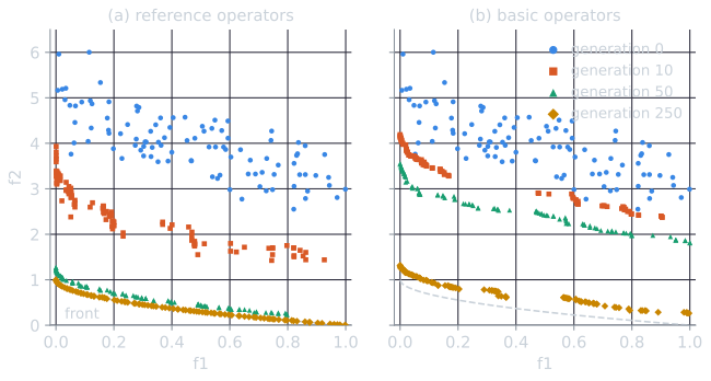
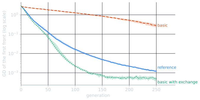
Medians and interquartile ranges at selected generations, rounded to three significant figures:
| Generation | Reference | Basic | Basic with exchange |
|---|---|---|---|
| 0 | 2.76 (2.69 to 2.84) | 2.76 (2.69 to 2.84) | 2.76 (2.69 to 2.84) |
| 25 | 0.449 (0.421 to 0.495) | 2.15 (2.05 to 2.23) | 0.352 (0.331 to 0.376) |
| 50 | 0.124 (0.105 to 0.144) | 1.81 (1.72 to 1.91) | 0.0679 (0.0574 to 0.0875) |
| 100 | 0.0162 (0.0144 to 0.0185) | 1.29 (1.20 to 1.35) | 0.00228 (0.00207 to 0.00254) |
| 250 | 0.00124 (0.00115 to 0.00140) | 0.278 (0.225 to 0.340) | 0.000525 (0.000371 to 0.000629) |
The three variants start from the same random populations, so they agree at generation 0. By generation 25 the basic operators have reduced GD by about a fifth, and the other two by a factor of six or more.
Adding only the exchange closed the whole gap: the basic operators with exchange did as well as the reference operators, slightly better in GD. So on these problems the bounded form of the distributions was not needed to reach the reference results, and the random assignment of values to children was. A likely explanation is this. Without the exchange, SBX with $\eta_c = 20$ makes children that are near-copies of their parents, each variable moved only slightly toward or away from the other parent's value, so progress toward $g = 1$ falls largely to mutation, which changes about one variable per child. With the exchange, each child takes about half of its crossed variables from the other parent's side, a recombination much like uniform crossover, and good values of different variables, found in different individuals, can be combined. The ZDT functions reward this, since $g$ is a sum over separate variables. The small edge of the basic-with-exchange variant may come from clipping, which places children exactly on the bound $x_i = 0$ where the optimum lies.
The exchange is easiest to see with two variables. The script nsga2_trace.py crosses the parents $p_1 = (0.2, 0.7)$ and $p_2 = (0.7, 0.2)$ 4,000 times with $\eta_c = 20$, each variable crossed with probability 0.5 as in the experiment, and records the first child before mutation.
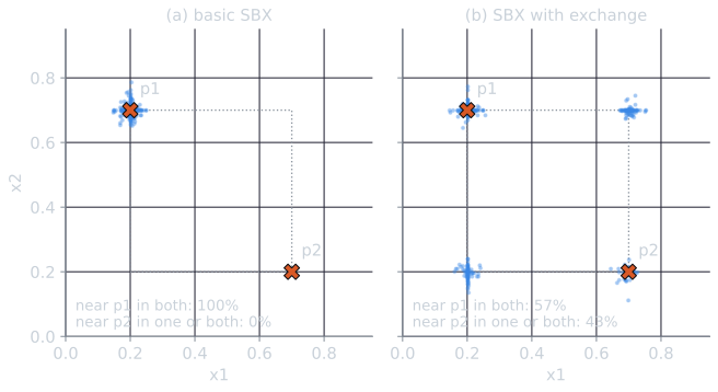
Without the exchange, every child lay nearer $p_1$ than $p_2$ in both variables, and 26% were exact copies of $p_1$, the crossings in which neither variable was crossed. With it, 57% lay nearer $p_1$ in both variables, 37% took one variable from the $p_2$ side, and 7% took both. These are close to the values expected when each variable independently ends up on the $p_2$ side with probability $0.5 \times 0.5 = 0.25$: $0.75^2 = 56\%$, $2 \times 0.75 \times 0.25 = 38\%$ and $0.25^2 = 6\%$, rounded. In 30 dimensions the same mechanism moves about a quarter of the variables of a crossed pair to the other parent's side, which is what lets good values found in different individuals meet in one.
Comparison with the paper
The paper reports the mean and variance of $\Upsilon$ and $\Delta$ over 10 runs (Deb et al., 2002, Tables II and III). Means are compared here:
| Problem | $\Upsilon$, paper real-coded | $\Upsilon$, paper binary | $\Upsilon$, ours (reference) | $\Delta$, paper real-coded | $\Delta$, paper binary | $\Delta$, ours (reference) |
|---|---|---|---|---|---|---|
| ZDT1 | 0.033482 | 0.000894 | 0.001572 | 0.390307 | 0.463292 | 0.3817 |
| ZDT2 | 0.072391 | 0.000824 | 0.001462 | 0.430776 | 0.435112 | 0.3831 |
| ZDT3 | 0.114500 | 0.043411 | 0.001172 | 0.738540 | 0.575606 | 0.5524 |
Three cautions apply. First, $\Upsilon$ depends on how the 500 reference points are placed, which the paper describes only as uniform, and it cannot reach zero: even the ideal set scores 0.000734 on ZDT1 with our placement, so values near 0.001 mean essentially converged in both studies. Second, the two studies did not necessarily use the same operator code; the paper predates the 2005 release of the reference code. Third, the paper's runs are 10 and ours 30.
With those cautions, our $\Upsilon$ is of the same order as the paper's binary-coded results on ZDT1 and ZDT2 and lower on ZDT3, our $\Delta$ is close to or below the paper's values, and our runs converged far better than the paper's real-coded runs. The real-coded $\Upsilon$ of 0.033 to 0.115 lies between our reference and basic results, and the experiment cannot say which implementation details produced it. What it does show is that the paper's settings, $N = 100$, 250 generations, $\eta_c = \eta_m = 20$, $p_c = 0.9$ and $p_m = 1/n$, are not a complete specification of the algorithm's behaviour: in this implementation, whether each crossed variable's two new values are assigned to the children in random order, an implementation detail that the paper never mentions, changes the median GD on ZDT1 by more than two orders of magnitude.
Limitations
The crowding distance is computed one objective at a time, from each solution's two neighbours in that objective. With two objectives this approximates the spacing along the front well. With many objectives, a solution's neighbours in different objectives are different solutions, and the estimate becomes a poor guide to density. Non-dominated sorting also loses its discriminating power, since most of a population becomes non-dominated. These difficulties motivated NSGA-III, which keeps the NSGA-II framework but replaces crowding with reference points (Deb and Jain, 2014). Other open issues are those of the whole family: the result is a set, and how good a set is depends on the indicator used to judge it, as Pareto-optimal ranking of optimizers discusses.
References
- Deb, K., and Agrawal, R. B. (1995). Simulated binary crossover for continuous search space. Complex Systems, 9(2), 115–148.
- Deb, K., and Jain, H. (2014). An evolutionary many-objective optimization algorithm using reference-point-based nondominated sorting approach, Part I: Solving problems with box constraints. IEEE Transactions on Evolutionary Computation, 18(4), 577–601.
- Deb, K., Pratap, A., Agarwal, S., and Meyarivan, T. (2002). A fast and elitist multiobjective genetic algorithm: NSGA-II. IEEE Transactions on Evolutionary Computation, 6(2), 182–197.
- Knowles, J. D., and Corne, D. W. (2000). Approximating the nondominated front using the Pareto archived evolution strategy. Evolutionary Computation, 8(2), 149–172.
- Srinivas, N., and Deb, K. (1994). Multiobjective optimization using nondominated sorting in genetic algorithms. Evolutionary Computation, 2(3), 221–248.
- Zitzler, E., Deb, K., and Thiele, L. (2000). Comparison of multiobjective evolutionary algorithms: Empirical results. Evolutionary Computation, 8(2), 173–195.
- Zitzler, E., and Thiele, L. (1999). Multiobjective evolutionary algorithms: A comparative case study and the strength Pareto approach. IEEE Transactions on Evolutionary Computation, 3(4), 257–271.