Consider a two-variable problem that has served as a benchmark for constrained evolutionary algorithms since the 1990s. It asks for the minimum of $f(x) = (x_1 - 10)^3 + (x_2 - 20)^3$ over the box $13 \le x_1 \le 100$, $0 \le x_2 \le 100$, subject to two constraints: the point must lie outside the circle of radius 10 around $(5, 5)$ and inside the circle of radius 9.1 around $(6, 5)$. The feasible region is the thin crescent between the two circles, and it covers 0.0067% of the box. A population of 50 points scattered uniformly over the box contains no feasible point at all with probability 0.997. The objective, meanwhile, keeps decreasing toward the corner $(13, 0)$, which lies just outside the crescent. An evolutionary algorithm (EA) that knows only the objective will find that corner, not the answer.
Most real optimization problems have constraints of this kind: capacities, budgets, physical limits, compatibility rules. They pose a particular difficulty for EAs, because the variation operators are blind to them. Two feasible parents can have an infeasible child, and nothing in mutation or crossover knows where the feasible region is (Eiben and Smith, 2015, ch. 13). Constraint handling is the set of techniques that decide what the algorithm does with infeasible candidates. This article describes the main families, then compares several of them on the problem above.
The constrained problem
A constrained optimization problem asks to
$$\text{minimize } f(x) \quad \text{subject to} \quad g_j(x) \le 0, \; j = 1, \dots, J, \qquad h_k(x) = 0, \; k = 1, \dots, K,$$
with $x$ in a box of lower and upper bounds. The feasible region is the set of points satisfying every constraint. Bounds are usually easy to enforce directly, by clipping or by sampling within them. The other constraints are the hard part. Equality constraints are commonly relaxed to inequalities $\lvert h_k(x) \rvert - \varepsilon \le 0$ for a small tolerance $\varepsilon$, since a randomly varied point almost never satisfies an equality exactly (Coello Coello, 2002).
Most methods measure how far a point is from feasibility by its constraint violation,
$$\mathrm{CV}(x) = \sum_{j=1}^{J} \max\big(0,\, g_j(x)\big),$$
with equality constraints included in their relaxed form. $\mathrm{CV}(x) = 0$ exactly when $x$ is feasible. Since constraints are often measured in different units, they are usually normalized first, for example by dividing each one by a constant of its own size, so that no single constraint dominates the sum.
In the mid-1990s, Michalewicz and Schoenauer (1996) surveyed the evolutionary methods proposed for such problems, found the experimental results on many test cases disappointing, and proposed a set of eleven test cases for future comparisons. Surveys of that period sorted the methods into four categories: preserving feasibility, penalty functions, searching for feasibility, and hybrids (Koziel and Michalewicz, 1999). Koziel and Michalewicz added decoders as a fifth. Coello Coello (2002) gave a longer survey, organized as penalty functions, special representations and operators, repair algorithms, separation of objectives and constraints, and hybrid methods. The sections below follow roughly that order.
Penalty functions
The most common approach turns the constrained problem into an unconstrained one by adding a penalty for violation:
$$F(x) = f(x) + R \cdot P(x),$$
where $P(x) \ge 0$ measures the violation and is zero for feasible points, and $R > 0$ is a weight. The EA then minimizes $F$ as if there were no constraints. A common choice of $P$ is the quadratic loss $\sum_j \max(0, g_j(x))^2$ (Runarsson and Yao, 2000); another is the linear sum $\mathrm{CV}(x)$.
The difficulty is the choice of $R$. If it is too small, infeasible points with good objective values score better than feasible ones, and the algorithm converges to an infeasible solution. If it is too large, any feasible point beats every infeasible one, which discourages the algorithm from exploring through infeasible regions and makes it hard to move between separate feasible regions (Runarsson and Yao, 2000). Where the constrained optimum lies on the boundary of the feasible region, as it usually does, there is a further subtlety from classical optimization. The minimizer of a quadratic penalty function generally differs from the constrained solution for every finite weight, so the penalized optimum is slightly infeasible however large $R$ is. A linear penalty is exact: if $x^*$ is a strict local solution that satisfies the usual first-order conditions and $R$ exceeds the largest of its Lagrange multipliers, then $x^*$ is a local minimizer of $f + R \cdot \mathrm{CV}$ (Nocedal and Wright, 2006, §17.2). The multipliers are not known in advance, so the threshold is not either. Both effects appear in the experiment below.
Both effects in one variable
A problem small enough to solve by hand shows both effects exactly. Minimize
$$f(x) = (x - 2)^2 \quad \text{subject to} \quad g(x) = x - 1 \le 0.$$
Without the constraint the minimum is at $x = 2$; with it, the best feasible point is the boundary $x^* = 1$, where $f = 1$. The Lagrange multiplier $\lambda$ at $x^*$ measures how strongly the objective pulls against the constraint: the first-order condition $f'(x^*) + \lambda g'(x^*) = 0$ gives $2(1 - 2) + \lambda = 0$, so $\lambda = 2$. Equivalently, relaxing the constraint to $x \le 1 + \epsilon$ would lower the optimal objective by about $2\epsilon$.
Quadratic penalty. For $x > 1$ the penalized objective is $F(x) = (x - 2)^2 + R (x - 1)^2$. Setting $F'(x) = 2(x - 2) + 2R(x - 1) = 0$ gives
$$x_R = \frac{2 + R}{1 + R} = 1 + \frac{1}{1 + R},$$
which lies to the right of 1, in the infeasible region, for every finite $R$. The violation $1/(1 + R)$ shrinks as the weight grows but never reaches zero. The reason is visible in the derivative: the slope of the penalty term, $2R(x - 1)$, is zero at $x = 1$, so the penalty cannot resist the objective's pull, $f'(1) = -2$, until $x$ has moved past the boundary.
Linear penalty. For $x > 1$, $F(x) = (x - 2)^2 + R(x - 1)$ and $F'(x) = 2(x - 2) + R$, which is zero at $x = 2 - R/2$. That point lies to the right of 1 only if $R < 2$. If $R \ge 2$, then $F'(x) > 0$ for every $x > 1$, so $F$ increases away from the boundary and the minimizer is $x^* = 1$ exactly. The threshold is the multiplier: the penalty's constant slope $R$ must at least match the objective's pull $\lambda = 2$ at the boundary.
| $R$ | Quadratic $x_R$ | Violation | Linear $x_R$ | Violation |
|---|---|---|---|---|
| 0.5 | 1.6667 | 0.6667 | 1.7500 | 0.7500 |
| 1 | 1.5000 | 0.5000 | 1.5000 | 0.5000 |
| 2 | 1.3333 | 0.3333 | 1.0000 | 0 |
| 4 | 1.2000 | 0.2000 | 1.0000 | 0 |
| 10 | 1.0909 | 0.0909 | 1.0000 | 0 |
| 100 | 1.0099 | 0.0099 | 1.0000 | 0 |
The values come from the closed forms above, checked by a grid search, in tools/experiments/evolution/constraint_examples.py (rounded to four decimals).
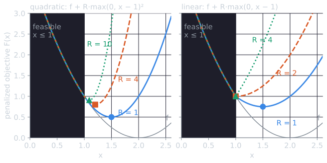
The linear penalty pays for exactness with a kink at the boundary, where $F$ is not differentiable. That is a difficulty for gradient-based optimizers, and none for an evolutionary algorithm, which compares function values only.
Static, dynamic and adaptive penalties
The variants differ in how they set $R$.
Static penalties keep the weights fixed for the whole run. Homaifar, Qi, and Lai (1994) defined several levels of violation for each constraint, each level with its own coefficient that grows with the level. The method needs many parameters, $m(2l + 1)$ for $m$ constraints and $l$ levels according to Coello Coello (2002), and their values depend on the problem.
The death penalty rejects infeasible points outright, in effect giving them infinite penalty. It is simple and costs nothing to compute, and it has been popular with evolution strategies. It is limited to problems whose feasible region is convex and a reasonably large part of the search space, and it uses no information from infeasible points. If the initial population contains no feasible point, all candidates are equally bad and the search has nothing to follow (Coello Coello, 2002).
Dynamic penalties make the weight a function of the generation number $t$. Joines and Houck (1994) evaluated individuals with
$$F(x) = f(x) + (C\, t)^{\alpha} \sum_j \max\big(0, g_j(x)\big)^{\beta},$$
with $C = 0.5$ and $\alpha, \beta \in \{1, 2\}$ in their experiments. The penalty starts mild, letting the population explore infeasible regions, and grows until infeasible points cannot compete. The results were sensitive to $\alpha$ and $\beta$, and settings that worked for the authors led to premature convergence on other problems (Coello Coello, 2002).
Adaptive penalties adjust the weight using feedback from the search. In the scheme of Ben Hadj-Alouane and Bean (1997), the weight $\lambda(t)$ is divided by a factor $\beta_1 > 1$ if the best individual of each of the last $k$ generations was feasible, multiplied by $\beta_2 > 1$ if it was infeasible in each of them, and left unchanged otherwise, with $\beta_1 \ne \beta_2$ to avoid cycling. If the search keeps finding only feasible solutions, the penalty is presumably larger than needed. If it keeps finding only infeasible ones, it is too small.
Deb's feasibility rules
Deb (2000) removed the penalty weight altogether by observing that tournament selection never needs a fitness value, only a decision about which of two individuals is better. In a binary tournament between two solutions, his method applies three rules:
- A feasible solution is preferred to an infeasible one.
- Of two feasible solutions, the one with the better objective value is preferred.
- Of two infeasible solutions, the one with the smaller constraint violation is preferred.
Equivalently, each individual receives the fitness
$$F(x) = \begin{cases} f(x) & \text{if } x \text{ is feasible,} \\ f_{\text{worst}} + \mathrm{CV}(x) & \text{otherwise,} \end{cases}$$
for minimization, where $f_{\text{worst}}$ is the objective value of the worst feasible solution in the current population, or zero if there is none. Every infeasible individual then ranks below every feasible one, and infeasible individuals are ranked among themselves by violation alone, without any reference to the objective. No weight is needed. Deb normalized the constraints so that violations of different constraints are comparable (Coello Coello, 2002).
Deb's rules on six points
Take six points of the benchmark problem from the introduction, g06, which is defined in full in the worked example below. Three lie in the feasible crescent; three do not. D is the corner $(13, 0)$ that the unconstrained objective prefers, and F lies a hair outside the crescent next to the optimum. Violations use the normalized constraints $g_1/100$ and $g_2/82.81$ of the experiment, and values are rounded as shown:
| Point | $(x_1, x_2)$ | $f(x)$ | $\mathrm{CV}(x)$ | Feasible | $F(x)$ under Deb's rules |
|---|---|---|---|---|---|
| A | (14.2, 1.07) | −6709.38 | 0 | yes | −6709.38 |
| B | (15.0, 5.0) | −3250.00 | 0 | yes | −3250.00 |
| C | (14.5, 1.8) | −5937.44 | 0 | yes | −5937.44 |
| D | (13.0, 0.0) | −7973.00 | 0.1100 (all $g_1$) | no | −3249.8900 |
| E | (14.0, 0.0) | −7936.00 | 0.0747 (all $g_2$) | no | −3249.9253 |
| F | (14.095, 0.85) | −6954.07 | 0.0006 (all $g_1$) | no | −3249.9994 |
The worst feasible objective value is B's, so $f_{\text{worst}} = -3250$, and each infeasible point's fitness is $-3250$ plus its violation. Some tournaments:
- A against C: both feasible, so the lower objective wins, A (rule 2).
- B against F: B is feasible and F is not, so B wins (rule 1), although F's objective is better by more than 3,700 and its violation is tiny.
- D against E: both infeasible, so the smaller violation wins, E (rule 3), although D has the better objective.
- E against F: both infeasible, and F wins on violation.
Sorting by $F$ ranks the six as A, C, B, F, E, D: the feasible points by objective, then the infeasible ones by violation. A static quadratic penalty $f + R \sum_j \max(0, g_j)^2$ ranks them by a single number whose meaning depends on $R$. With $R = 10^2$ it ranks D, E, F, A, C, B, all three infeasible points first, because the penalties (at most $10^2 \times 0.11^2 = 1.21$) are tiny next to differences in $f$ of hundreds. With $R = 10^6$ it ranks F, A, C, B, E, D: D and E are now heavily penalized, but F's penalty, $10^6 \times 0.00058^2 \approx 0.34$, is still smaller than its lead in objective over A, so the infeasible F is ranked best. Only with $R = 10^{10}$ does the penalty ranking put the feasible A and C first, as A, C, F, B, E, D, and F still beats the feasible B. Deb's rules reach a feasibility-first ranking with no weight at all.
The rules push the population toward the feasible region first and toward the optimum second. Their weakness is the same infinite preference for feasibility. A population can collapse onto the first feasible region it finds and lose the diversity it needs to improve. Deb's method relied on niching to maintain diversity, and Coello Coello (2002) noted that niching combined with higher than usual mutation rates appears necessary to avoid stagnation. The same principle, under the name constrained domination, governs the selection of the multi-objective algorithm NSGA-II (Deb, Pratap, Agarwal, and Meyarivan, 2002), and the bin-packing genetic algorithm written for this course used the same three rules, with the number of overfilled bins as the violation.
Stochastic ranking
Runarsson and Yao (2000) looked at the choice between objective and penalty as a question of which one dominates the comparison of two individuals. A large penalty weight means that comparisons involving infeasible individuals are decided almost always by the penalty, a small one that they are decided almost always by the objective. Stochastic ranking makes that balance explicit with a single probability $P_f$.
The population is ranked by a procedure like bubble sort. In each sweep, adjacent individuals are compared in turn. If both are feasible, they are compared by objective value. Otherwise, with probability $P_f$ they are compared by objective value, and with probability $1 - P_f$ by penalty, here the quadratic loss. The worse individual of each pair moves down. Sweeps repeat up to $\lambda$ times for a population of $\lambda$, and stop early if a whole sweep changes nothing. Selection then takes the top of the ranking. With $P_f = 0$ the ranking is the over-penalized one, which, like Deb's rules, places every feasible individual above every infeasible one. With $P_f$ close to 1 the constraints are ignored in comparisons involving infeasible individuals. Runarsson and Yao argued that $P_f$ should be below $1/2$ to bias the search against infeasible solutions, and they used $P_f = 0.45$.
Here is the procedure on the six points of the previous section, with $P_f = 0.45$ and the quadratic loss as penalty (0 for A, B and C; 0.0121 for D, 0.0056 for E, $3.4 \times 10^{-7}$ for F). The initial order is random, as in Runarsson and Yao's procedure; with seed 1 of the script it is E, A, C, B, F, D. Each comparison draws a uniform number $u$; if both individuals are feasible, or if $u < 0.45$, they are compared by $f$, otherwise by penalty.
| Comparison | $u$ | Compared by | Result | Order afterwards |
|---|---|---|---|---|
| E, A | 0.31 | $f$ ($u < 0.45$) | E's −7936 beats A's −6709: keep | E A C B F D |
| A, C | 0.42 | $f$ (both feasible) | keep | E A C B F D |
| C, B | 0.83 | $f$ (both feasible) | keep | E A C B F D |
| B, F | 0.41 | $f$ ($u < 0.45$) | F's −6954 beats B's −3250: swap | E A C F B D |
| B, D | 0.55 | penalty | B's 0 beats D's 0.0121: keep | E A C F B D |
A second sweep, with fresh draws, changes nothing, so the procedure stops with the ranking E, A, C, F, B, D. The infeasible E is ranked first because its single comparison happened to be decided by the objective. The ranking is random by design, and its tendency shows only over many draws: over seeds 0 to 999 the feasible A is ranked first 505 times and in the top three 88% of the time, while the infeasible D, which has the best objective and the largest violation, is first 105 times and has a mean rank of 4.01. In the algorithm the ranking is redone every generation and the top $\mu$ of $\lambda$ individuals are kept, so infeasible individuals with good objective values survive often enough to guide the search, without dominating it.
They tested the method inside a $(30, 200)$ evolution strategy on thirteen benchmark problems, g01 to g13, with 30 runs per problem and at most $200 \times 1{,}750 = 350{,}000$ evaluations per run. On g06, the problem of the introduction, it found the optimum in 20 of the 30 runs, with mean $-6875.940$, while the decoder-based method of Koziel and Michalewicz (1999) reported a mean of $-6342.6$ and never found the optimum. Their broader conclusion was that suitable ranking alone, without specialized variation operators, improved performance significantly on their benchmarks.
Repair, decoders and feasibility-preserving operators
Penalties and ranking rules keep infeasible individuals in the population and judge them. The remaining families avoid judging them, by turning them into feasible ones or by never producing them.
Repair maps an infeasible individual to a nearby feasible one, usually with a problem-specific heuristic: drop items from an overfull knapsack, move a clashing exam to a free slot. The repaired version is evaluated. A design question is whether it also replaces the original in the population, which makes the search Lamarckian. Coello Coello (2002) reports a rule of thumb from combinatorial problems, that replacing about 5% of the originals with their repaired versions works best, and a 15% rule reported for numerical problems with nonlinear constraints. Repair works well when a cheap repair heuristic exists, and it can bias the search when the heuristic always lands in the same part of the feasible region.
A decoder changes the representation so that every genotype maps to a feasible solution. The chromosome becomes a set of instructions for building a solution rather than the solution itself. For bin packing, a permutation of the items, decoded by placing each item in turn into the first bin with room for it, always gives a feasible packing, and the EA searches over permutations. Koziel and Michalewicz (1999) built a general decoder for continuous problems, a homomorphous mapping from an $n$-dimensional cube onto the feasible region. Coello Coello (2002) noted its costs: an extra parameter, a binary search for the boundary of the feasible region at each decoding, and a loss of locality on non-convex regions, where a small change in the cube can produce a large change in the decoded point.
Feasibility-preserving operators keep the population feasible by construction. If the constraint is that a tour visits every city exactly once, a tour represented as a permutation and changed only by operators that turn permutations into permutations never violates it. More generally, initializing inside the feasible region and using operators that are closed over it, such as arithmetic crossover over a convex region, keeps every individual feasible. Both decoders and preserving operators depend on knowing the structure of the feasible region, which is why they are effective where they apply and unavailable for constraints that are known only through a black-box function.
A worked example: g06
The problem of the introduction is g06 in the numbering of Runarsson and Yao (2000), also part of the CEC 2006 benchmark suite (Liang et al., 2006):
$$\begin{aligned} \text{minimize}\quad & f(x) = (x_1 - 10)^3 + (x_2 - 20)^3 \\ \text{subject to}\quad & g_1(x) = -(x_1 - 5)^2 - (x_2 - 5)^2 + 100 \le 0, \\ & g_2(x) = (x_1 - 6)^2 + (x_2 - 5)^2 - 82.81 \le 0, \\ & 13 \le x_1 \le 100, \quad 0 \le x_2 \le 100. \end{aligned}$$
Both constraints are active at the optimum, which is the lower intersection of the two circles. Setting $g_1 = g_2 = 0$ and subtracting gives $(x_1 - 5)^2 - (x_1 - 6)^2 = 100 - 82.81$, that is $2x_1 - 11 = 17.19$, so $x_1^* = 14.095$. Then $x_2^* = 5 - \sqrt{100 - 9.095^2} = 0.8429608$, and $f(x^*) = -6961.81388$.
The script tools/experiments/evolution/constraints.py in the site repository checks these values and compares constraint-handling methods on this problem. Constraints are normalized as $g_1 / 100$ and $g_2 / 82.81$, and $\mathrm{CV}$ is the sum of their positive parts. Of $10^7$ points drawn uniformly from the box, 675 were feasible, a fraction of 0.0067%. The unconstrained minimum over the box is at the corner $(13, 0)$, with $f = -7973$ and normalized violation 0.11 of the first constraint. The Lagrange multipliers of the two normalized constraints at $x^*$ are about $1.10 \times 10^5$ and $1.02 \times 10^5$, so a linear penalty $f + R \cdot \mathrm{CV}$ is guaranteed to be exact for $R$ above about $1.1 \times 10^5$.
All methods share one real-coded genetic algorithm and differ only in how two individuals are compared. The population of 50 is initialized uniformly in the box. Parents are chosen by 50 binary tournaments (see selection pressure and premature convergence). Pairs of parents undergo simulated binary crossover (Deb and Agrawal, 1995; see crossover and mutation operators) with probability 0.9 and distribution index 15, and each variable of each child undergoes polynomial mutation with probability 0.5 and distribution index 20. The children replace the parents, except that the best individual of the previous generation replaces the worst child. Each run lasts 1,000 generations, or 50,050 evaluations, and returns the best individual of its final population by its own comparison rule. Each method was run with the same 30 seeds.
| Method | Runs returning a feasible point | $f$ of feasible returns, median (IQR) | Infeasible returns: median $f$, median CV |
|---|---|---|---|
| Deb's rules | 30 of 30 | −6910.58 (−6932.68 to −6897.00) | none |
| Quadratic penalty, $R = 10^2$ | 0 of 30 | −7973.00, 0.11 | |
| Quadratic penalty, $R = 10^4$ | 0 of 30 | −7953.54, 0.011 | |
| Quadratic penalty, $R = 10^6$ | 0 of 30 | −7952.18, 0.010 | |
| Quadratic penalty, $R = 10^8$ | 0 of 30 | −7070.96, 0.0010 | |
| Quadratic penalty, $R = 10^{10}$ | 24 of 30 | −6935.68 (−6947.24 to −6922.72) | −6952.78, $6.9 \times 10^{-6}$ |
| Linear penalty, $R = 10^4$ | 0 of 30 | −7953.22, 0.0098 | |
| Linear penalty, $R = 10^5$ | 0 of 30 | −7553.91, 0.0057 | |
| Linear penalty, $R = 10^6$ | 28 of 30 | −6923.49 (−6937.71 to −6908.39) | −6960.35, $1.5 \times 10^{-5}$ |
| Death penalty | 24 of 30 | −6752.42 (−6824.56 to −6368.93) | 82,462.81, 33.8 |
Several points stand out.
Penalty weights span many orders of magnitude. The quadratic penalty needed a weight of $10^{10}$ before most runs returned a feasible point. Below that, every run converged on an infeasible point with an objective value better than the true optimum, and the algorithm did exactly what it was asked to do: it minimized $F$. With $R = 10^2$ the runs returned the corner $(13, 0)$ itself. For weights from $10^4$ to $10^6$, they returned points on the bottom edge $x_2 = 0$, near $x_1 = 13.6$. These points lie just inside the first circle (and, at $R = 10^6$, also just outside the second), violating the constraints by about 1% of their scale in total, and their objective values are almost 1,000 units better than the optimum. The linear penalty behaved as the exactness threshold predicts: at $R = 10^5$, just below the multipliers, no run was feasible, and at $R = 10^6$, 28 of 30 were.
Large weights still return slightly infeasible points. The infeasible returns at the largest weights violate the constraints by about $10^{-5}$, and their objective values, −6952.78 and −6960.35, beat the feasible optimum. Whether such a point counts as a solution depends on the tolerance the application allows. In a benchmark that requires exact feasibility, it does not.
Deb's rules needed no tuning and were feasible in every run, but did not reach the optimum. The median returned value, −6910.58, was 51 above $f^*$, and no run of any method came within 1 of it within this budget. Once the population was inside the crescent, the rules discarded any child that stepped outside it, and the crescent is narrowest near the optimum. This is the loss of diversity that Deb addressed with niching, which this experiment did not include.
The death penalty is random search until a feasible point appears. With no feasible point in the initial population, every tournament between two infeasible points is a tie. The six runs that never stumbled on the crescent returned an arbitrary infeasible point, and the others could begin to improve only once one of their children had landed in it.
The GA found the penalized minimum
Were the penalty runs a failure of the search or of the penalty? The question can be settled without any evolution, by minimizing the penalized objective $F$ directly with a numerical optimizer for each weight (L-BFGS-B from five starting points for the quadratic penalty, a refined grid search for the linear penalty, whose kinks defeat gradient methods; constraint_examples.py, rounded as shown).
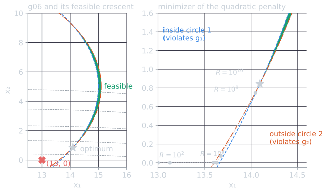
| Weight $R$ | Minimizer of $f + R \sum_j \max(0, g_j)^2$ | $f$ there | CV there | Predicted CV, $\sum_j \lambda_j / (2R)$ |
|---|---|---|---|---|
| $10^2$ | (13.0000, 0.0000) | −7973.00 | 0.11 | |
| $10^4$ | (13.5949, 0.0000) | −7953.54 | 0.0113 | |
| $10^6$ | (13.6296, 0.0000) | −7952.18 | 0.0101 | |
| $10^7$ | (13.6747, 0.0730) | −7863.07 | 0.0092 | |
| $10^8$ | (14.0474, 0.7467) | −7070.75 | 0.0010 | 0.0011 |
| $10^9$ | (14.0902, 0.8330) | −6972.99 | $1.06 \times 10^{-4}$ | $1.06 \times 10^{-4}$ |
| $10^{10}$ | (14.0945, 0.8420) | −6962.94 | $1.06 \times 10^{-5}$ | $1.06 \times 10^{-5}$ |
| $10^{12}$ | (14.0950, 0.8430) | −6961.83 | $1.13 \times 10^{-7}$ | $1.06 \times 10^{-7}$ |
For $R = 10^4$ and $10^6$ the minimizer is exactly where the GA runs converged, with the same objective value to the second decimal (−7953.54 and −7952.18), and for $R = 10^8$ the GA's median, −7070.96, is within a fraction of a unit of the minimizer's −7070.75. The GA solved the problem it was given. The penalty function defined the wrong problem.
The last column comes from the first-order condition at the minimizer. Where both constraints are violated, the gradient of $F$ is $\nabla f + \sum_j 2R\, g_j \nabla g_j = 0$. At the constrained optimum, the Karush-Kuhn-Tucker condition reads $\nabla f + \sum_j \lambda_j \nabla g_j = 0$. When $x_R$ is close to $x^*$ the gradients are nearly the same, so the two conditions match when $2R\, g_j \approx \lambda_j$, that is
$$g_j(x_R) \approx \frac{\lambda_j}{2R}.$$
Each violation falls in proportion to $1/R$, exactly as in the one-variable example, where $\lambda = 2$ and the violation was $1/(1 + R)$. With the multipliers $1.10 \times 10^5$ and $1.02 \times 10^5$, the prediction is accurate from $R = 10^8$ on; below that, $x_R$ is too far from $x^*$ for the approximation, and the bound $x_1 \ge 13$ and the edge $x_2 = 0$ take over. To get the violation below $10^{-6}$, the weight must exceed about $10^{11}$, at which point the penalty term is so large that tiny violations dominate every comparison, which is exactly the situation in which, as Runarsson and Yao (2000) observed, the search loses the ability to cross infeasible regions.
The linear penalty's minimizer, found the same way, is infeasible for $R = 10^4$, $3 \times 10^4$, $10^5$ and $1.05 \times 10^5$ (at $10^5$ it is $(13.837, 0.375)$ with $f = -7502.12$ and $\mathrm{CV} = 0.0052$, close to the GA's infeasible returns at that weight) and is the optimum itself from $1.1 \times 10^5$ on, just above the larger multiplier, $1.097 \times 10^5$. The threshold that the theory predicts shows up between $1.05 \times 10^5$ and $1.1 \times 10^5$, where the multiplier says it should.
These numbers describe one plain genetic algorithm on one problem at one budget. They should not be read as a ranking of the methods. Runarsson and Yao (2000) reached the optimum in two-thirds of their runs with an evolution strategy, self-adapted step sizes and seven times the budget. The lessons that do carry over concern the mechanisms: the weight of a penalty is a real parameter with a threshold that depends on the problem, quadratic penalties are never exact, and comparison rules that put feasibility first trade tuning for a risk of stagnation.
References
- Ben Hadj-Alouane, A., and Bean, J. C. (1997). A genetic algorithm for the multiple-choice integer program. Operations Research, 45(1), 92–101.
- Coello Coello, C. A. (2002). Theoretical and numerical constraint-handling techniques used with evolutionary algorithms: A survey of the state of the art. Computer Methods in Applied Mechanics and Engineering, 191(11–12), 1245–1287.
- Deb, K. (2000). An efficient constraint handling method for genetic algorithms. Computer Methods in Applied Mechanics and Engineering, 186(2–4), 311–338.
- Deb, K., and Agrawal, R. B. (1995). Simulated binary crossover for continuous search space. Complex Systems, 9(2), 115–148.
- Deb, K., Pratap, A., Agarwal, S., and Meyarivan, T. (2002). A fast and elitist multiobjective genetic algorithm: NSGA-II. IEEE Transactions on Evolutionary Computation, 6(2), 182–197.
- Eiben, A. E., and Smith, J. E. (2015). Introduction to Evolutionary Computing, 2nd ed., chapter 13. Springer.
- Homaifar, A., Qi, C. X., and Lai, S. H. (1994). Constrained optimization via genetic algorithms. Simulation, 62(4), 242–253.
- Joines, J. A., and Houck, C. R. (1994). On the use of non-stationary penalty functions to solve nonlinear constrained optimization problems with GA's. In Proceedings of the First IEEE Conference on Evolutionary Computation, 579–584. IEEE.
- Koziel, S., and Michalewicz, Z. (1999). Evolutionary algorithms, homomorphous mappings, and constrained parameter optimization. Evolutionary Computation, 7(1), 19–44.
- Liang, J. J., Runarsson, T. P., Mezura-Montes, E., Clerc, M., Suganthan, P. N., Coello Coello, C. A., and Deb, K. (2006). Problem definitions and evaluation criteria for the CEC 2006 special session on constrained real-parameter optimization. Technical report, Nanyang Technological University, Singapore.
- Michalewicz, Z., and Schoenauer, M. (1996). Evolutionary algorithms for constrained parameter optimization problems. Evolutionary Computation, 4(1), 1–32.
- Nocedal, J., and Wright, S. J. (2006). Numerical Optimization, 2nd ed., section 17.2. Springer.
- Runarsson, T. P., and Yao, X. (2000). Stochastic ranking for constrained evolutionary optimization. IEEE Transactions on Evolutionary Computation, 4(3), 284–294.