A steel beam of circular cross-section is clamped to a wall at one end and carries a load of 1 kN at the other. The designer chooses its diameter and its length, and wants the beam both light and stiff: low weight, and little deflection at the loaded end. A beam 20 mm thick and 200 mm long weighs 0.490 kg and deflects 1.640 mm. A beam 30 mm thick and 200 mm long weighs 1.103 kg and deflects 0.324 mm. Neither design is better than the other. The first is lighter, the second stiffer, and choosing between them requires knowing how much a kilogram is worth in millimetres, which the problem statement does not say. A third design, 25 mm by 300 mm, weighs 1.149 kg and deflects 2.267 mm. It is worse than the first beam in both respects, and no statement of preferences could make it the right choice.
This is the situation of multi-objective optimization: several objectives that conflict, so that improving one costs something in another. A single-objective method can rank any two candidates, as a hill climber or a genetic algorithm does every time it compares fitness values. With several objectives, some pairs of candidates cannot be ranked at all. The concept that replaces the ranking is Pareto dominance, and the solutions it leaves unbeaten form the Pareto-optimal set. This article defines both precisely, following Deb (2001), Miettinen (1999), and Eiben and Smith (2015, ch. 12), and works through the beam design problem from Deb (2001).
Decision space and objective space
A multi-objective optimization problem asks to
$$\text{minimize } \mathbf{f}(\mathbf{x}) = \big(f_1(\mathbf{x}), f_2(\mathbf{x}), \dots, f_M(\mathbf{x})\big) \quad \text{subject to } \mathbf{x} \in S,$$
where $\mathbf{x} = (x_1, \dots, x_n)$ is a vector of $n$ decision variables and $S$ is the feasible set: the points within the variable bounds that satisfy every constraint. Objectives to be maximized are negated, so minimization loses no generality. Two spaces are involved. The decision space is where $\mathbf{x}$ lives, here the pairs (diameter, length). The objective space is where $\mathbf{f}(\mathbf{x})$ lives, here the pairs (weight, deflection). The image $Z = \mathbf{f}(S)$ is the set of attainable objective vectors (Miettinen, 1999, Part I, §2.1).
The distinction matters because the two spaces have different geometry. Two designs can be far apart in decision space and close in objective space, or the reverse, and the shape of $Z$ (convex, curved, broken into pieces) decides which solution methods work. Comparisons between solutions happen entirely in objective space. Search operators such as mutation and crossover act in decision space.
Dominance
For two objective vectors $\mathbf{a} = \mathbf{f}(\mathbf{x})$ and $\mathbf{b} = \mathbf{f}(\mathbf{y})$, all objectives minimized, three relations are standard. Names vary across the literature. This article follows Zitzler, Thiele, Laumanns, Fonseca, and da Fonseca (2003).
- $\mathbf{a}$ weakly dominates $\mathbf{b}$, written $\mathbf{a} \preceq \mathbf{b}$, if $a_i \le b_i$ for every $i$: it is no worse in any objective.
- $\mathbf{a}$ dominates $\mathbf{b}$, written $\mathbf{a} \prec \mathbf{b}$, if $a_i \le b_i$ for every $i$ and $a_j < b_j$ for at least one $j$: no worse in any objective and strictly better in at least one.
- $\mathbf{a}$ strictly dominates $\mathbf{b}$ if $a_i < b_i$ for every $i$: better in every objective.
Each relation in the list implies the one above it: strict dominance implies dominance, which implies weak dominance. Two vectors are incomparable when neither weakly dominates the other. The middle relation is the one usually meant by "dominates" without qualification, and it is the two-condition test that Deb (1999) states: no worse in all objectives, strictly better in at least one.
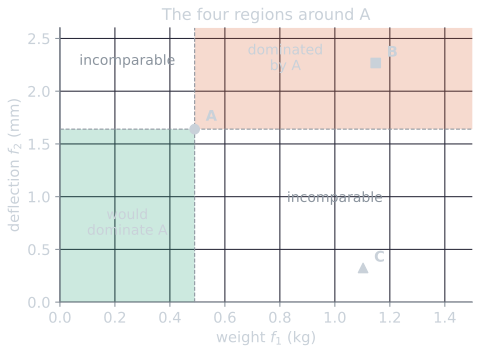
In the opening example, call the three beams $A$ (20 mm by 200 mm), $B$ (25 by 300) and $C$ (30 by 200). $A$ strictly dominates $B$, since it is lighter and stiffer. $C$ also strictly dominates $B$. $A$ and $C$ are incomparable.
A picture makes the definitions concrete. Draw a vertical and a horizontal line through $\mathbf{a}$ in objective space. They cut the plane into four quadrants. Every point in the upper-right quadrant, its boundary included, is no better than $\mathbf{a}$ in either objective, so $\mathbf{a}$ dominates it (unless it is $\mathbf{a}$ itself). Every point in the lower-left quadrant would dominate $\mathbf{a}$. Points in the other two quadrants are better in one objective and worse in the other, and so are incomparable with $\mathbf{a}$. With two objectives, half of the plane around any point is incomparable with it. With $M$ objectives, only two of the $2^M$ orthants around a point are ordered with respect to it, the one where every objective is better and the one where every objective is worse, so the incomparable share grows quickly with the number of objectives. This is one reason why problems with many objectives are hard for dominance-based algorithms, as multi-objective evolutionary algorithms discusses.
Dominance is a strict partial order on objective vectors. It is transitive (if $\mathbf{a} \prec \mathbf{b}$ and $\mathbf{b} \prec \mathbf{c}$ then $\mathbf{a} \prec \mathbf{c}$) and irreflexive (no vector dominates itself), but it is not complete: unlike the order on real numbers, it leaves many pairs unordered. That incompleteness is the whole difficulty of the subject. Every concept below is a way of living with it.
The Pareto-optimal set and front
A feasible point $\mathbf{x}^* \in S$ is Pareto optimal if no feasible point dominates it: there is no $\mathbf{x} \in S$ with $\mathbf{f}(\mathbf{x}) \prec \mathbf{f}(\mathbf{x}^*)$. Equivalently, no objective can be improved without making at least one other worse. The set of all Pareto-optimal points is the Pareto-optimal set, which lies in decision space. Its image in objective space, $\{\mathbf{f}(\mathbf{x}^*)\}$, is the Pareto-optimal front (Deb, 2001; Miettinen, 1999, Part I, §2.2). Miettinen (1999) speaks of Pareto optimal decision vectors and Pareto optimal objective vectors. Both usages are common.
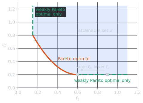
A weaker notion is also needed. A point is weakly Pareto optimal if no feasible point strictly dominates it, that is, no point is better in every objective at once (Miettinen, 1999, Part I, §2.5). Every Pareto-optimal point is weakly Pareto optimal, but not conversely. If part of the attainable set has a flat edge, where one objective can fall while the other stays constant, the points along that edge other than its best end are weakly Pareto optimal but not Pareto optimal: some other point is better in one objective and equal in the other. Several scalarization methods, discussed in weighted sums and the ε-constraint method, are guaranteed only to return weakly Pareto-optimal points, so the distinction has practical weight.
The Pareto-optimal set is defined against all of $S$. An algorithm sees only the points it has evaluated. Among a finite set of points, those that no other member dominates form the non-dominated set of that sample. It is the algorithm's best estimate of the front, but it is not the front: a point can be non-dominated among the points found so far and still be dominated by a point not yet found (Deb, 1999). For two objectives and distinct points, the non-dominated set of $N$ points is found by sorting on $f_1$, breaking ties by $f_2$, and scanning: a point is non-dominated exactly when its $f_2$ is lower than that of every point before it. The general case compares every pair, at cost $O(MN^2)$ for $M$ objectives. Repeating the extraction on the remaining points sorts a population into successive fronts, the idea behind NSGA-II.
The scan is correct for a simple reason. After sorting, any point that could dominate $\mathbf{p}$ has $f_1$ no larger than $p_1$, so it comes before $\mathbf{p}$; the tie-break on $f_2$ puts a point with equal $f_1$ and lower $f_2$ first as well. An earlier point $\mathbf{q}$ already has $q_1 \le p_1$, so it dominates $\mathbf{p}$ exactly when $q_2 \le p_2$. Keeping track of the lowest $f_2$ seen so far is therefore enough: $\mathbf{p}$ survives if its $f_2$ is strictly below that running minimum.
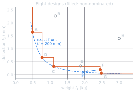
A worked scan. Add five more beams to $A$, $B$ and $C$, all feasible, and label them $D$ to $H$. The script tools/experiments/evolution/pareto_scan.py computes their objectives (rounded to four decimals) and runs the scan. In order of weight:
| Design | $d$, $l$ (mm) | Weight (kg) | Deflection (mm) | Lowest deflection before it | Result |
|---|---|---|---|---|---|
| A | 20, 200 | 0.4901 | 1.6402 | none | non-dominated |
| D | 25, 200 | 0.7658 | 0.6718 | 1.6402 | non-dominated |
| C | 30, 200 | 1.1027 | 0.3240 | 0.6718 | non-dominated |
| B | 25, 300 | 1.1486 | 2.2675 | 0.3240 | dominated |
| E | 35, 250 | 1.8761 | 0.3416 | 0.3240 | dominated |
| F | 40, 250 | 2.4504 | 0.2002 | 0.3240 | non-dominated |
| G | 45, 200 | 2.4811 | 0.0640 | 0.2002 | non-dominated |
| H | 35, 400 | 3.0018 | 1.3991 | 0.0640 | dominated |
One pass over the sorted list keeps A, D, C, F and G. A check of all 28 pairs agrees: B is dominated by A, C and D; E only by C, which is lighter and, by 0.0176 mm, stiffer; and H by C, D, E, F and G. The interesting row is F. It is non-dominated among these eight designs, yet it is not Pareto optimal: the beam of the same diameter at the shortest length, 40 mm by 200 mm, weighs 1.9604 kg and deflects 0.1025 mm, and dominates it. The non-dominated set of a sample is an estimate of the front, and F is where the estimate is wrong. The interactive demo in quality indicators for Pareto fronts marks the non-dominated members of any point set as points are added and dragged.
The cantilever beam, worked
Deb (2001) states the beam problem as follows. A solid circular beam of diameter $d$ and length $l$ carries an end load $P$. The objectives are its weight and its end deflection,
$$f_1(d, l) = \rho \frac{\pi d^2}{4} l, \qquad f_2(d, l) = \delta = \frac{64 P l^3}{3 E \pi d^4},$$
subject to two constraints: the maximum bending stress $\sigma_{\max} = 32 P l / (\pi d^3)$ must not exceed the strength $S_y$, and the deflection must not exceed $\delta_{\max}$. The deflection and stress are the textbook formulas for an end-loaded cantilever, $\delta = P l^3 / (3 E I)$ and $\sigma = M c / I$, with second moment of area $I = \pi d^4 / 64$, bending moment $M = P l$ at the wall, and $c = d/2$. The data are $\rho = 7800$ kg/m³, $P = 1$ kN, $E = 207$ GPa, $S_y = 300$ MPa, $\delta_{\max} = 5$ mm, $10 \le d \le 50$ mm and $200 \le l \le 1000$ mm. Working in newtons and millimetres keeps the units straight: $P = 1000$ N, $E = 207{,}000$ N/mm², and stress comes out in N/mm², which is MPa.
Where the front is. For a fixed diameter, weight grows with $l$, deflection with $l^3$, and stress with $l$. Shortening a feasible beam therefore makes it lighter, stiffer and less stressed, so any feasible design with $l > 200$ mm is strictly dominated by the same diameter at $l = 200$ mm. Along $l = 200$ mm, weight grows with $d$ and deflection falls with $d$, so no two of those designs dominate each other. The Pareto-optimal set is the segment $l = 200$ mm, $d_{\min} \le d \le 50$ mm, where $d_{\min}$ is the smallest diameter that satisfies both constraints at that length. The stress limit requires $d^3 \ge 32 P l / (\pi S_y)$, so $d \ge 18.937$ mm. The deflection limit requires only $d \ge 15.136$ mm. Stress is the binding constraint, and $d_{\min} = 18.937$ mm.
On that segment the diameter can be eliminated, which gives the front in closed form. The weight equation gives $d^2 = 4 f_1 / (\rho \pi l)$, so $d^4 = 16 f_1^2 / (\rho^2 \pi^2 l^2)$. Substituting into the deflection,
$$f_2 = \frac{64 P l^3}{3 E \pi} \cdot \frac{\rho^2 \pi^2 l^2}{16 f_1^{\,2}} = \frac{4 \pi P \rho^2 l^5}{3 E} \cdot \frac{1}{f_1^{\,2}}.$$
With $l = 200$ mm, $\rho = 7.8 \times 10^{-6}$ kg/mm³, $P = 1000$ N and $E = 207{,}000$ N/mm², the constant is $4\pi \times 1000 \times (7.8 \times 10^{-6})^2 \times 200^5 / (3 \times 207{,}000) = 0.3940$ kg²·mm, so
$$f_2 = \frac{0.3940}{f_1^{\,2}} \quad (f_1 \text{ in kg}, \ f_2 \text{ in mm}), \qquad 0.4394 \le f_1 \le 3.0631.$$
The curve is convex, and it runs from the lightest feasible beam (0.4394 kg, deflecting 2.0409 mm) to the stiffest (3.0631 kg, deflecting 0.0420 mm). Taking logarithms, $\log f_2 = \log 0.3940 - 2 \log f_1$: on logarithmic axes the front is a straight line of slope $-2$, which is how the figure below draws it.
What sampling finds. The script tools/experiments/evolution/pareto_basics.py in the site repository draws 10,000 designs uniformly from the box (seed 1). Of these, 4,005 (40.1%) are feasible; 5,855 satisfy the stress limit and 4,108 the deflection limit. Among the feasible designs, 39 are non-dominated. Their lengths run from 200.0 to 210.8 mm, close to the exact $l = 200$ mm, and their diameters from 19.31 to 49.46 mm. At equal weight, their deflection exceeds the exact front's by a median of 5.3% and at most 30.1%. A selection:
| $d$ (mm) | $l$ (mm) | Weight (kg) | Deflection (mm) |
|---|---|---|---|
| 19.31 | 201.7 | 0.4608 | 1.9345 |
| 24.70 | 202.7 | 0.7576 | 0.7339 |
| 29.16 | 205.9 | 1.0729 | 0.3960 |
| 37.34 | 202.1 | 1.7258 | 0.1392 |
| 45.05 | 201.4 | 2.5048 | 0.0651 |
| 49.46 | 201.9 | 3.0262 | 0.0451 |
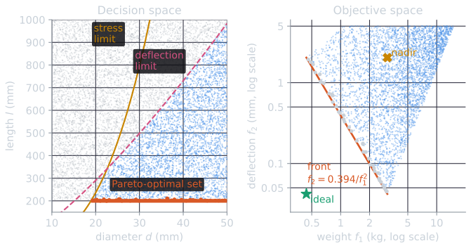
The two panels show the same designs through the map $\mathbf{f}$. A thin strip of decision space, lengths from 200 to 210.8 mm, holds every non-dominated sample, and the whole two-dimensional feasible region folds onto a wedge of objective space whose lower-left edge is the front. The Pareto-optimal set here is a one-dimensional segment inside a two-dimensional box, and a search must first find that segment, then spread its points along it.
Random sampling found the right region but not the front itself, and it spent 60% of its evaluations on infeasible designs. Getting close to the front, and spreading points along it, is the job of the algorithms in multi-objective evolutionary algorithms.
Ideal and nadir points
Two reference vectors summarize the extent of the front. The ideal point $\mathbf{z}^{\text{ideal}}$ has as its $i$-th component the minimum of $f_i$ over the feasible set, each objective minimized on its own. The nadir point $\mathbf{z}^{\text{nad}}$ has as its $i$-th component the maximum of $f_i$ over the Pareto-optimal set, the worst value of each objective among the efficient solutions (Miettinen, 1999, Part I, §2.4). Together they bound the front: every Pareto-optimal objective vector lies in the box between them. A utopian point is the ideal point moved slightly below in every component, so that it is strictly better than every attainable vector, which some methods require.
For the beam, the ideal point is (0.4394 kg, 0.0420 mm) and the nadir point is (3.0631 kg, 2.0409 mm). The ideal point is not attainable: no beam is both as light as the lightest and as stiff as the stiffest. If it were attainable, the objectives would not conflict and the front would be a single point.
The ideal point is easy to compute, since it takes $M$ single-objective optimizations. The nadir point is harder. With two objectives, the nadir is read off the two ends of the front, as here. With three or more, the usual estimate from the table of objective values at the $M$ single-objective optima (the payoff table) can be wrong in either direction, because the worst value of an objective over the front need not occur at another objective's optimum (Miettinen, 1999, Part I, §2.4.2). Both points are used to normalize objectives to comparable ranges, $(f_i - z_i^{\text{ideal}}) / (z_i^{\text{nad}} - z_i^{\text{ideal}})$, before weighting them or measuring distances between them. Without normalization, the beam's weights in kilograms and deflections in millimetres would be compared as if one unit of each were worth the same.
Local and global Pareto optimality
Single-objective search has local optima, points that no small move improves but that are not the best overall, as escaping local optima discusses. Multi-objective search has the same phenomenon. A point $\mathbf{x}^*$ is locally Pareto optimal if there is a neighborhood of $\mathbf{x}^*$ in which no feasible point dominates it (Miettinen, 1999, Part I, §2.2). Pareto optimality over the whole feasible set is then called global for contrast. Every globally Pareto-optimal point is locally Pareto optimal; for convex problems the converse also holds (Miettinen, 1999, Part I, §2.2), but not in general.
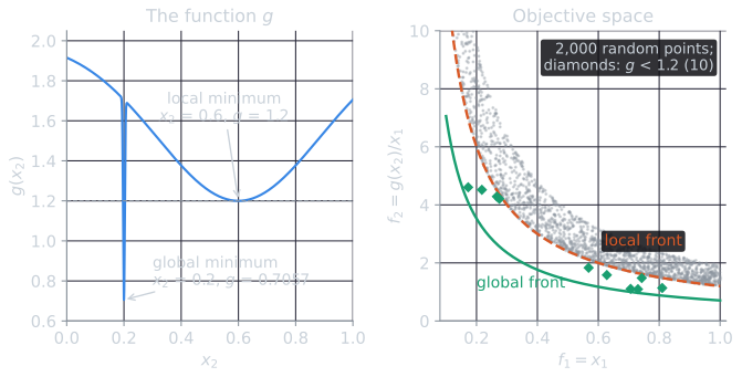
Deb (1999) built a test problem that shows the difference:
$$f_1 = x_1, \qquad f_2 = \frac{g(x_2)}{x_1}, \qquad g(x_2) = 2 - \exp\left[-\left(\frac{x_2 - 0.2}{0.004}\right)^2\right] - 0.8 \exp\left[-\left(\frac{x_2 - 0.6}{0.4}\right)^2\right],$$
with $0.1 \le x_1 \le 1$ and $0 \le x_2 \le 1$. For a fixed $x_1$, the smaller $g(x_2)$, the better $f_2$, while $f_1$ is unchanged, so the Pareto-optimal points are those where $x_2$ minimizes $g$. The function $g$ has a broad local minimum at $x_2 = 0.6$, where $g = 1.2$, and a narrow global minimum at $x_2 = 0.2$, where $g = 0.7057$. Each gives a front of the form $f_2 = c / f_1$: a local front with $c = 1.2$, and the global front with $c = 0.7057$. The point $(x_1, x_2) = (0.5, 0.6)$, with objectives (0.5, 2.4), has no dominating neighbor within 0.05 in either variable, checked on a grid of 40,400 neighbors by the same script. It is locally Pareto optimal. The point (0.5, 0.2), with objectives (0.5, 1.4114), dominates it, so it is not globally Pareto optimal. Only values of $x_2$ between 0.1967 and 0.2033, 0.66% of the range, give $g$ below 1.2, so a search that samples $x_2$ broadly will find the local front much more often than the global one. Of 2,000 points drawn uniformly from the box (seed 3, in pareto_scan.py), 10 land in that narrow valley; the other 1,990 lie on or above the local front. That is the purpose of the construction: Deb (1999) showed how to carry difficulties such as multimodality and deception from single-objective functions into multi-objective test problems through the function $g$. The ZDT test problems of Zitzler, Deb, and Thiele (2000) follow the same pattern.
A short history
The idea is older than optimization as a discipline. In Mathematical Psychics, Edgeworth (1881) analyzed exchange between two parties using indifference curves and identified the contract curve, the set of allocations from which neither party can gain without the other losing. Pareto (1906), in the Manuale di economia politica, defined the maximum of welfare, or "ophelimity", for a community as a position from which every small move raises the ophelimity of some members and lowers that of others. The name "Pareto optimality" was attached to the concept later. Stadler (1979) surveys its history from 1776 to 1960, following the related ideas of efficiency, the vector maximum problem and Pareto optimality through economics, production theory and mathematical programming. Evolutionary algorithms took the concept up much later, in the population-based methods that Deb (2001) reviews.
The trade-off view of decision making
Pareto optimality does not pick a solution. It removes the solutions that no reasonable decision maker would pick and leaves a set of candidates that only preferences can separate. Along the beam's front, the price of stiffness rises steeply: from the closed form, going from 1.0 to 1.1 kg reduces the deflection from 0.394 to 0.326 mm, while going from 2.0 to 2.1 kg reduces it from 0.098 to 0.089 mm. The same 100 g buys about 7.5 times less stiffness at the heavy end (0.0684 mm against 0.0092 mm; the unrounded ratio is 7.47). The derivative of the closed form makes the rule exact: $\mathrm{d}f_2 / \mathrm{d}f_1 = -2 \times 0.3940 / f_1^{\,3}$, which is $-0.788$ mm per kg at 1 kg and $-0.0985$ mm per kg at 2 kg. Doubling the weight divides the marginal gain in stiffness by $2^3 = 8$. The slope of the front at a point is the local rate of exchange between the objectives: how many millimetres of deflection a kilogram of added steel removes, or, read the other way, how much weight a millimetre less deflection costs there. A designer who sees this curve can choose with that knowledge; a designer who sees only one point cannot.
Methods differ in when the preferences enter. In a priori methods the decision maker states preferences first, for example as weights, and the problem is reduced to a single objective. In a posteriori methods the front, or a representative set of points on it, is generated first and the decision maker chooses from it. In interactive methods the two alternate (Miettinen, 1999, Part II). Scalarization methods, treated in weighted sums and the ε-constraint method, solve one single-objective problem per point. Evolutionary algorithms suit the a posteriori approach because a population can carry many non-dominated points at once and approximate the whole front in a single run, without assumptions about its shape (Deb, 2001; Eiben and Smith, 2015, ch. 12). How well an approximation does that is measured by indicators such as those in hypervolume and generational distance, and it is the subject of the rest of the multi-objective optimization topic.
References
- Deb, K. (1999). Multi-objective genetic algorithms: Problem difficulties and construction of test problems. Evolutionary Computation, 7(3), 205–230.
- Deb, K. (2001). Multi-Objective Optimization Using Evolutionary Algorithms. John Wiley & Sons.
- Edgeworth, F. Y. (1881). Mathematical Psychics: An Essay on the Application of Mathematics to the Moral Sciences. C. Kegan Paul.
- Eiben, A. E., and Smith, J. E. (2015). Introduction to Evolutionary Computing, 2nd ed., chapter 12. Springer.
- Miettinen, K. (1999). Nonlinear Multiobjective Optimization. Kluwer Academic Publishers.
- Pareto, V. (1906). Manuale di economia politica. Società Editrice Libraria.
- Stadler, W. (1979). A survey of multicriteria optimization or the vector maximum problem, part I: 1776–1960. Journal of Optimization Theory and Applications, 29(1), 1–52.
- Zitzler, E., Deb, K., and Thiele, L. (2000). Comparison of multiobjective evolutionary algorithms: Empirical results. Evolutionary Computation, 8(2), 173–195.
- Zitzler, E., Thiele, L., Laumanns, M., Fonseca, C. M., and da Fonseca, V. G. (2003). Performance assessment of multiobjective optimizers: An analysis and review. IEEE Transactions on Evolutionary Computation, 7(2), 117–132.