A single-objective evolutionary algorithm needs one number per individual: its fitness. Selection compares those numbers, and the population moves toward the best. With two or more conflicting objectives, say cost and weight of a bracket, each individual has a vector instead, and two vectors often cannot be ordered. A light, expensive bracket and a heavy, cheap one are both reasonable answers. The goal is no longer a single optimum but the whole set of Pareto-optimal trade-offs, so that a designer can choose among them afterwards.
A population is well suited to this goal, since it can hold many trade-offs at once and find them in one run, instead of the one-at-a-time solutions of weighted sums and ε-constraints. What it needs is a way to turn objective vectors into selection decisions. Every multi-objective evolutionary algorithm (MOEA) answers three questions:
- Fitness assignment. How are vectors turned into a preference between individuals? This determines whether the population moves toward the Pareto front, the convergence goal.
- Diversity. What keeps the population spread along the front rather than collapsed onto one part of it? This is the spread goal.
- Elitism. Are good non-dominated solutions protected from being lost by chance?
The history of the field, surveyed in Eiben and Smith (2015, ch. 12), is largely a sequence of better answers to these three questions. This article follows that sequence. The most widely used of these algorithms, NSGA-II, has its own article with a full specification and an experiment.
To make the answers comparable, the article applies several of them to one small population, the nine designs of the NSGA-II article, each scored on two objectives to be minimized:
| Design | A | B | C | D | E | F | G | H | I |
|---|---|---|---|---|---|---|---|---|---|
| $(f_1, f_2)$ | (1, 8) | (2, 5) | (4, 4) | (6, 2) | (9, 1) | (3, 7) | (5, 5) | (7, 3) | (8, 6) |
A to E are mutually non-dominated. B dominates F, G and I; C dominates G and I; D dominates H and I; G and H each dominate I. The script tools/experiments/evolution/moea_comparison.py in the site repository computes every value quoted for this example below.
Selecting one objective at a time: VEGA
The usual starting point of the history is Schaffer's vector evaluated genetic algorithm (VEGA), presented in 1985. VEGA changes only selection. With $q$ objectives and population size $N$, it fills $q$ subpopulations of size $N/q$, each by fitness-proportional selection on one objective alone, shuffles them together, and then applies crossover and mutation as usual (Schaffer, 1985; Fonseca and Fleming, 1993).
The weakness is that no individual is ever selected for being a good compromise. Fonseca and Fleming (1993) pointed out, after Richardson and colleagues, that shuffling the subpopulations together is equivalent to selecting on a weighted sum of the objectives, with weights that depend on the current population. Two non-dominated individuals are then generally sampled at different rates, and on some shapes of front the population tends to split into groups that each excel in one objective, which Schaffer had anticipated and called speciation. Horn, Nafpliotis and Goldberg (1994) summarized the experience: VEGA seems able to find only the extreme points of the front.
Pareto ranking with niching: MOGA, NPGA and NSGA
In his review of VEGA, Goldberg (1989) proposed the idea that shaped the next generation of algorithms: rank individuals by non-domination, so that selection depends only on Pareto dominance and not on any weighting, and add a niching method to keep the population from converging to a single point of the front. Three algorithms of 1993 and 1994 implemented the proposal in different ways. All three used fitness sharing or a relative of it, which divides an individual's fitness by a niche count of the neighbours within a radius $\sigma_{\text{share}}$.
MOGA (Fonseca and Fleming, 1993) gives each individual the rank
$$\text{rank}(x) = 1 + p(x),$$
where $p(x)$ is the number of individuals in the current population that dominate $x$. Non-dominated individuals have rank 1. Fitness is assigned by interpolating from the best rank to the worst, usually linearly, and then averaging the fitness of individuals that share a rank, so that all of them are sampled at the same rate. Sharing is applied in objective space, and the niche counts scale fitness within each rank, which spreads the population along the trade-off surface rather than across the decision variables.
NPGA, the niched Pareto genetic algorithm (Horn, Nafpliotis and Goldberg, 1994), replaces ranking with Pareto domination tournaments. Two candidates are drawn, together with a comparison set of $t_{\text{dom}}$ individuals. If one candidate is dominated by some member of the comparison set and the other is not, the other wins. Otherwise the tournament is a tie, and the candidate with the smaller niche count wins. $t_{\text{dom}}$ controls the domination pressure. On Schaffer's single-variable test problem, with $N = 30$, $t_{\text{dom}} = 4$ and $\sigma_{\text{share}} = 0.1$, NPGA maintained a fairly even spread of solutions along the front, stable for 200 generations.
NSGA, the non-dominated sorting genetic algorithm (Srinivas and Deb, 1994), sorts the population into fronts. The non-dominated individuals form the first front and all receive the same dummy fitness. Sharing on the decision vectors degrades that fitness within the front. The front is then set aside, the next non-dominated set is extracted and given a dummy fitness smaller than the smallest shared fitness of the front before, and so on until every individual is classified. The original study combined this with stochastic remainder selection (Zitzler and Thiele, 1999, summarize the procedure).
MOGA's ranks and NSGA's fronts usually agree on which individuals are best but not on how the rest are ordered. On the nine designs:
| Design | A | B | C | D | E | F | G | H | I |
|---|---|---|---|---|---|---|---|---|---|
| Dominated by | none | none | none | none | none | B | B, C | D | B, C, D, G, H |
| MOGA rank $1 + p(x)$ | 1 | 1 | 1 | 1 | 1 | 2 | 3 | 2 | 6 |
| NSGA front | 1 | 1 | 1 | 1 | 1 | 2 | 2 | 2 | 3 |
Both give A to E the best value. MOGA then separates G, which two designs dominate, from F and H, which one design each dominates, while NSGA puts all three on the second front, since each is non-dominated once the first front is set aside. I is the clearest case: five designs dominate it, so MOGA ranks it 6, three ranks below G, while NSGA places it only one front behind. A count of dominators measures how deeply an individual is buried in the population; a front index measures how many layers must be peeled away before it is exposed. Neither is more correct, but the choice changes the selection pressure on the dominated individuals.
These algorithms established Pareto ranking as the basis of fitness. Deb, Pratap, Agarwal and Meyarivan (2002) later named the three criticisms that NSGA had attracted, which apply to this whole generation: sorting that cost $O(MN^3)$ per generation for $M$ objectives and $N$ individuals, the lack of elitism, and the need to choose $\sigma_{\text{share}}$.
Elitism and archives: SPEA, PAES and SPEA2
A non-elitist algorithm can find a Pareto-optimal solution and lose it in the next generation. Zitzler, Deb and Thiele (2000) compared several algorithms on six test problems, now known as the ZDT problems, and concluded that elitism is an important factor in improving multi-objective search. The elitist algorithms of this period keep the best solutions found so far, either in a separate archive or by selecting survivors from parents and offspring together.
SPEA, the strength Pareto evolutionary algorithm (Zitzler and Thiele, 1999), keeps an external archive $P'$ of the non-dominated solutions found so far. Each archive member $i$ receives a strength
$$s_i = \frac{n_i}{N + 1},$$
where $n_i$ is the number of members of the population (of size $N$) that it covers, that is, dominates or equals. A population member $j$ receives the fitness
$$f_j = 1 + \sum_{i \in P',\ i \text{ covers } j} s_i,$$
to be minimized, and an archive member's fitness is its strength. Every archive member therefore has fitness below 1 and every population member at least 1. The scheme is also a niching method without a radius: an archive member that covers many population members has a high strength, which penalizes all of them, so individuals in crowded regions of the front are selected less often. Parents are chosen by binary tournaments from the population and archive together. When the archive grows beyond its maximum size, it is reduced by average-linkage clustering, the agglomerative method of hierarchical clustering, keeping one representative per cluster.
PAES, the Pareto archived evolution strategy (Knowles and Corne, 2000), is elitism in its simplest form: a single parent, a single mutant, and an archive. In the version Deb et al. (2002) summarize, a mutant that dominates its parent replaces it, and a dominated mutant is discarded, as in a hill climber. When neither dominates the other, the archive decides: a mutant that dominates archive members is accepted, and otherwise the less crowded of parent and mutant is preferred. Crowding is measured on a grid that divides objective space into cells and adapts to the archive's range.
SPEA2 (Zitzler, Laumanns and Thiele, 2001) revised SPEA in three ways. Fitness is finer grained: the strength $S(i)$ of every individual, in the population and archive together, is the number of individuals it dominates, and its raw fitness $R(i)$ is the sum of the strengths of the individuals that dominate it. Non-dominated individuals have $R(i) = 0$. A density term breaks ties among equal raw fitness:
$$D(i) = \frac{1}{\sigma_i^k + 2}, \qquad F(i) = R(i) + D(i),$$
where $\sigma_i^k$ is the distance in objective space to the $k$-th nearest neighbour, with $k$ the square root of the combined population and archive size. The 2 in the denominator keeps $D(i)$ below 1, so it never outweighs a difference in raw fitness. The archive has a fixed size: if there are too few non-dominated individuals it is filled with the best dominated ones, and if there are too many it is truncated by repeatedly removing the individual closest to its nearest neighbour, with ties broken by the second-nearest distance and so on.
Treating the nine designs as the combined population and archive gives $k = \sqrt{9} = 3$. The strengths are $S = 3$ for B (it dominates F, G and I), 2 for C and D, 1 for G and H, and 0 for the rest. Raw fitness adds up the strengths of an individual's dominators: $R(F) = S(B) = 3$, $R(G) = S(B) + S(C) = 5$, $R(H) = S(D) = 2$, and $R(I) = 3 + 2 + 2 + 1 + 1 = 9$. For the density of A, its distances to the other designs in objective space, in increasing order, are $\sqrt{5} \approx 2.236$ (to F), $\sqrt{10} \approx 3.162$ (to B) and $5$ (to C), so $\sigma_A^3 = 5$ and $D(A) = 1/(5 + 2) = 0.1429$. The list holds the distances to the other individuals, not the zero distance from A to itself, as the paper's note on building the lists says (Zitzler, Laumanns and Thiele, 2001, pp. 7 to 8); implementations that keep the zero would use the second-nearest neighbour here. In full, rounded to four decimals:
| Design | A | B | C | D | E | F | G | H | I |
|---|---|---|---|---|---|---|---|---|---|
| Strength $S$ | 0 | 3 | 2 | 2 | 0 | 0 | 1 | 1 | 0 |
| Raw fitness $R$ | 0 | 0 | 0 | 0 | 0 | 3 | 5 | 2 | 9 |
| $\sigma^3$ | 5.000 | 3.000 | 2.828 | 3.162 | 5.099 | 2.828 | 2.828 | 2.828 | 4.472 |
| Fitness $F = R + D$ | 0.1429 | 0.2000 | 0.2071 | 0.1937 | 0.1409 | 3.2071 | 5.2071 | 2.2071 | 9.1545 |
Fitness is minimized. The raw fitness orders the dominated designs as MOGA's ranks do, with one refinement: it separates H from F, which MOGA tied, because it weights each dominator by how much it dominates. D, which dominates H, has strength 2; B, which dominates F, has strength 3. The same weighting decides G: G is dominated by B and C, whose strengths sum to 5, so it ends up well behind F, whose single dominator is B. Among the non-dominated designs, where $R = 0$, only density matters, and the isolated extremes E and A come first, C and B, with close neighbours, last.
NSGA-II belongs to the same period. It answers the three criticisms of NSGA with a fast sorting procedure, the crowding distance in place of sharing, and survivor selection from parents and offspring combined. Its specification is in the NSGA-II article.
Decomposition: MOEA/D
The Pareto-based algorithms never scalarize the objectives. Zhang and Li (2007) took the opposite route and returned to classical scalarization, but solved many scalar problems at once. MOEA/D, the multi-objective evolutionary algorithm based on decomposition, starts from $N$ evenly spread weight vectors $\lambda^1, \dots, \lambda^N$, each defining a scalar subproblem. With the Tchebycheff approach, in minimization form, subproblem $j$ is
$$\min_x \; g^{te}(x \mid \lambda^j, z^*) = \max_{1 \le i \le M} \lambda^j_i \, \lvert f_i(x) - z^*_i \rvert,$$
where $z^*$ is the reference point of the best value seen for each objective. Unlike a weighted sum, which cannot reach points on non-convex parts of a front (see the weighted-sum article), every Pareto-optimal point is the optimum of some Tchebycheff subproblem. The paper also proposes a penalty-based boundary intersection (PBI) approach, which measures a point's distance along the direction of a weight vector and adds a penalty, controlled by a parameter $\theta$, for its distance from that direction.
On the nine designs, the best value of each objective is 1, so $z^* = (1, 1)$. Five weight vectors define five subproblems, and each subproblem's value for every design is the larger of its two weighted distances from $z^*$. For B $= (2, 5)$ and $\lambda = (0.5, 0.5)$, for example, $g^{te} = \max(0.5 \cdot 1, 0.5 \cdot 4) = 2$. Rounded to two decimals:
| $\lambda$ | A | B | C | D | E | F | G | H | I | Best |
|---|---|---|---|---|---|---|---|---|---|---|
| (0.1, 0.9) | 6.30 | 3.60 | 2.70 | 0.90 | 0.80 | 5.40 | 3.60 | 1.80 | 4.50 | E |
| (0.3, 0.7) | 4.90 | 2.80 | 2.10 | 1.50 | 2.40 | 4.20 | 2.80 | 1.80 | 3.50 | D |
| (0.5, 0.5) | 3.50 | 2.00 | 1.50 | 2.50 | 4.00 | 3.00 | 2.00 | 3.00 | 3.50 | C |
| (0.7, 0.3) | 2.10 | 1.20 | 2.10 | 3.50 | 5.60 | 1.80 | 2.80 | 4.20 | 4.90 | B |
| (0.9, 0.1) | 0.70 | 0.90 | 2.70 | 4.50 | 7.20 | 1.80 | 3.60 | 5.40 | 6.30 | A |
Each subproblem picks a different design, and together the five pick out the whole first front. A dominated design can never do strictly better than a design that dominates it, since it is no better in either term of the maximum, so the winners all come from the first front. The geometry explains which design wins. The level sets of $g^{te}$ are right-angled corners whose vertices lie on the line through $z^*$ along which the two weighted distances are equal, $\lambda_1 (f_1 - z^*_1) = \lambda_2 (f_2 - z^*_2)$. As the value grows, the corner slides outward from $z^*$ along that line, and the subproblem's winner is the first design the corner touches. For $\lambda = (0.5, 0.5)$ the line is the diagonal $f_1 = f_2$, and C $= (4, 4)$ lies on it. Note that the line runs in the direction $(1/\lambda_1, 1/\lambda_2)$, not along $\lambda$ itself: a large weight on $f_1$ pulls its subproblem toward small $f_1$. A weighted sum with the same weights picks B rather than C for $\lambda = (0.5, 0.5)$, since $(2 + 5)/2 = 3.5$ is less than $(4 + 4)/2 = 4$. In fact no weighted sum with positive weights picks C. C beats B only if $4\lambda_1 + 4\lambda_2 < 2\lambda_1 + 5\lambda_2$, that is $2\lambda_1 < \lambda_2$, and beats D only if $4\lambda_1 + 4\lambda_2 < 6\lambda_1 + 2\lambda_2$, that is $\lambda_2 < \lambda_1$, and both cannot hold. Geometrically, C lies above the segment from B to D, which passes through $(4, 3.5)$: it sits in a non-convex dent of the front, the case described in the weighted-sum article, and Tchebycheff reaches it where the weighted sum cannot.
The population holds one solution per subproblem, the best found so far. Each subproblem has a neighbourhood, the $T$ subproblems with the closest weight vectors, and the algorithm exploits the expectation that neighbouring subproblems have similar optima. In each generation, for each subproblem $j$:
- Pick two subproblems from the neighbourhood of $j$ at random and create a child $y$ from their current solutions.
- Update $z^*$ with $y$'s objective values.
- For each neighbour $k$ of $j$, replace $k$'s solution with $y$ if $y$ is at least as good for subproblem $k$.
- Add $y$ to an external archive of non-dominated solutions if no member dominates it, removing the members it dominates.
Diversity comes from the spread of the weight vectors rather than from a density estimate, and mating is restricted to neighbours. $T$ trades exploration against exploitation: too small, and parents are nearly identical; too large, and parents from distant subproblems produce children that are poor for the subproblem at hand. Zhang and Li reported that MOEA/D had a lower computational cost per generation than NSGA-II and performed better than or similarly to it and to the earlier MOGLS on multi-objective knapsack problems and continuous test problems.
Indicators as fitness: IBEA and SMS-EMOA
Every algorithm above pursues convergence and spread through separate mechanisms, and so each pursues an implicit and slightly different notion of a good front. Zitzler and Künzli (2004) proposed to state the goal explicitly as a quality indicator and select on it directly. Their IBEA (indicator-based evolutionary algorithm) uses a binary indicator $I(A, B)$ comparing two sets. The main example is the additive ε-indicator, the smallest amount by which every objective of $A$ must be shifted for $A$ to weakly dominate $B$:
$$I_{\varepsilon+}(A, B) = \min_{\varepsilon} \left\{ \forall x_2 \in B \;\, \exists x_1 \in A : f_i(x_1) - \varepsilon \le f_i(x_2) \text{ for } i = 1, \dots, n \right\}.$$
Each individual's fitness sums the indicator values of all others against it,
$$F(x_1) = \sum_{x_2 \in P \setminus \{x_1\}} -e^{-I(\{x_2\}, \{x_1\}) / \kappa},$$
to be maximized, where $\kappa > 0$ is a scaling factor. The exponential amplifies the influence of individuals that dominate $x_1$ over those that do not. Environmental selection removes the individual with the smallest fitness, updates the fitness of the rest, and repeats until the population is back to size. No separate diversity mechanism is needed. In the adaptive version, which scales the indicator values by their maximum absolute value, $\kappa = 0.05$ was used for all problems. The paper also defines a hypervolume-based indicator for the same scheme.
SMS-EMOA (Beume, Naujoks and Emmerich, 2007) selects on the hypervolume, the region of objective space that a set dominates, bounded by a reference point (see quality indicators for Pareto fronts). It is a steady-state $(\mu + 1)$ algorithm: each step creates one offspring, sorts the $\mu + 1$ individuals into non-dominated fronts as NSGA-II does, and discards the member of the worst front that contributes least hypervolume, the volume that would be lost if it were removed. The journal paper also develops a selection criterion based on the number of solutions that dominate each point. Hypervolume rewards convergence and spread in a single number, but it depends on the choice of reference point, and its cost grows quickly with the number of objectives, which limits hypervolume-based selection to problems with a few objectives.
One point must go: three answers
The differences between these philosophies are easiest to see in the smallest decision any of them makes. Suppose the population is the first front of the nine designs, A $= (1, 8)$, B $= (2, 5)$, C $= (4, 4)$, D $= (6, 2)$ and E $= (9, 1)$, all mutually non-dominated, and one must be discarded. Pareto ranking cannot help, since all five share rank 1. Each algorithm's diversity mechanism decides.
NSGA-II discards the most crowded design by crowding distance. A and E, the extremes, have infinite distance, and the interior distances are $d_B = 0.9464$, $d_C = 0.9286$ and $d_D = 1.0536$, so C goes.
SMS-EMOA discards the design whose exclusive hypervolume contribution is smallest. In two objectives, with the designs sorted by $f_1$, the contribution of an interior design is the rectangle between it and its two neighbours: for B it is $(f_1(C) - f_1(B)) \cdot (f_2(A) - f_2(B)) = 2 \cdot 3 = 6$. C contributes $2 \cdot 1 = 2$ and D $3 \cdot 2 = 6$. The extremes' contributions reach out to the reference point $r$. With $r = (10, 9)$, one unit beyond the worst value of each objective, A contributes $(2 - 1)(9 - 8) = 1$ and E contributes $(10 - 9)(2 - 1) = 1$, so an extreme goes, A and E tying. With $r = (11, 10)$, A, C and E tie at 2; with $r = (12, 11)$, the extremes contribute 3 each and C goes. The decision depends on the reference point, as discussed in quality indicators for Pareto fronts.
IBEA with the additive ε-indicator and $\kappa = 0.05$, in its adaptive form, first scales each objective to $[0, 1]$ over the population, giving A $= (0, 1)$, B $= (0.125, 0.5714)$, C $= (0.375, 0.4286)$, D $= (0.625, 0.1429)$ and E $= (1, 0)$. For single points, $I_{\varepsilon+}(\{x_2\}, \{x_1\}) = \max_i \big(f_i(x_2) - f_i(x_1)\big)$, the amount by which $x_2$ must improve to weakly dominate $x_1$. The largest absolute value among the pairs is $c = 1$ (between A and E), so the indicator values are divided by 1. A's fitness collects one term from each other design:
$$F(A) = -\left(e^{-0.125/0.05} + e^{-0.375/0.05} + e^{-0.625/0.05} + e^{-1/0.05}\right) = -(0.0821 + 0.0006 + 0.0000 + 0.0000) = -0.0826.$$
The first term dominates: B needs to improve by only 0.125 in $f_1$ to cover A, so A adds little that B does not already offer. The fitness values are $-0.0826$ for A, $-0.0070$ for B, $-0.0642$ for C, $-0.0040$ for D and $-0.0576$ for E. The smallest is A's, so IBEA discards A.
| Design | Crowding distance | HV contribution, $r = (10, 9)$ | IBEA fitness |
|---|---|---|---|
| A | $\infty$ | 1 | $-0.0826$ |
| B | 0.9464 | 6 | $-0.0070$ |
| C | 0.9286 | 2 | $-0.0642$ |
| D | 1.0536 | 6 | $-0.0040$ |
| E | $\infty$ | 1 | $-0.0576$ |
| Discarded | C | A or E | A |
On five points, NSGA-II and IBEA disagree outright, and the hypervolume sides with either one depending on the reference point. NSGA-II protects the extremes unconditionally and judges interior points by the gap around them. The hypervolume weighs the area each point alone secures, so it values B and D, which hold large rectangles, and treats the extremes according to the reference point. The ε-indicator asks how cheaply each point could be replaced by another, and A, a small step from B, is the cheapest. Each choice encodes a different preference about what a good front looks like, which is the point Zitzler and Künzli (2004) made in proposing to state that preference explicitly.
Three spreads on the same problems
Repeated over a whole run, these small decisions shape the final front. The script moea_comparison.py runs NSGA-II, MOEA/D with the Tchebycheff approach, and the adaptive IBEA with the additive ε-indicator on ZDT1, whose front is convex, and ZDT2, whose front is concave (both are defined in the NSGA-II article). A population of 20 makes the spacing of the points easy to see. All three use the same variation operators, the bounded SBX and polynomial mutation of the NSGA-II reference code, with distribution indices of 20 and a mutation probability of $1/30$ per variable, and each runs for 1,000 generations, 20,020 evaluations. (At 250 generations none of the three had converged with so small a population.) MOEA/D uses 20 evenly spaced weight vectors, neighbourhoods of $T = 5$, crossover on every mating, and no external archive, the simple variant of Zhang and Li (2007, Section V-C). Their experiments used $T = 20$, a fifth of a population of 100 (Section V-E); here each neighbourhood is a quarter of the population. IBEA uses $\kappa = 0.05$ and creates 20 offspring per generation. Each algorithm was run with 30 seeds; the figure shows the run with the median hypervolume.
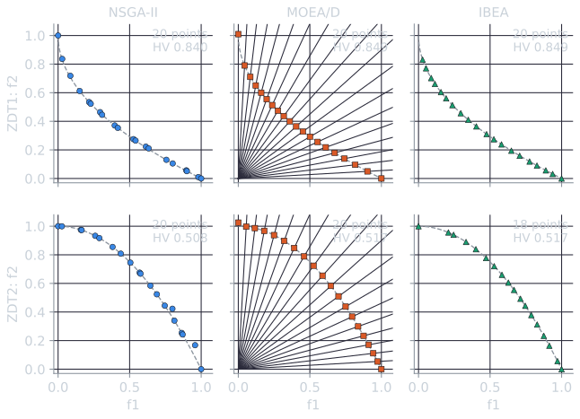
The median (and interquartile range) of four indicators over the 30 runs, on the non-dominated members of the final population (HV with reference point $(1.1, 1.1)$), rounded to three significant figures, GD to two; for scale, 20 points evenly spaced by arc length along the true front score HV 0.852 and IGD 0.0195 on ZDT1, and HV 0.520 and IGD 0.0195 on ZDT2:
| Problem | Algorithm | HV | IGD | Spacing | GD |
|---|---|---|---|---|---|
| ZDT1 | NSGA-II | 0.840 (0.838 to 0.842) | 0.0264 (0.0252 to 0.0277) | 0.0433 (0.0384 to 0.0483) | 0.0029 (0.0016 to 0.0041) |
| ZDT1 | MOEA/D | 0.849 (0.848 to 0.849) | 0.0243 (0.0237 to 0.0253) | 0.0423 (0.0407 to 0.0452) | 0.00052 (0.00012 to 0.0013) |
| ZDT1 | IBEA | 0.849 (0.848 to 0.851) | 0.0249 (0.0233 to 0.0267) | 0.0189 (0.0166 to 0.0226) | 0.000041 (0.000037 to 0.000045) |
| ZDT2 | NSGA-II | 0.508 (0.505 to 0.510) | 0.0275 (0.0261 to 0.0288) | 0.0432 (0.0398 to 0.0515) | 0.0035 (0.0021 to 0.0049) |
| ZDT2 | MOEA/D | 0.517 (0.516 to 0.518) | 0.0201 (0.0199 to 0.0204) | 0.0219 (0.0205 to 0.0233) | 0.00098 (0.00028 to 0.0020) |
| ZDT2 | IBEA | 0.517 (0.516 to 0.517) | 0.0248 (0.0242 to 0.0258) | 0.0389 (0.0337 to 0.0434) | 0.000035 (0.000031 to 0.000037) |
Spacing is Schott's measure, the standard deviation of the distances from each point to its nearest neighbour, so smaller is more even (see quality indicators). Three observations stand out. First, NSGA-II has the least even spacing on both problems and the largest GD. Once the population is close to the front, the first front of the 40 parents and offspring usually holds more than 20 members, and survivor selection removes the excess in one pass by crowding distance. The distances are computed once, before any member is removed, and are not updated as members go, so both members of a close pair can be removed together, leaving a hole, while another close pair survives intact. Second, MOEA/D's spread is set in advance by its weight vectors, and on ZDT2 it is the most even of the three, with the best IGD. On both problems the subproblem with weight $(1, 0)$ only asks for the smallest $f_1$, whatever $f_2$, so its solution need not converge in the other variables: in the runs shown, the first point lies 0.0096 above the ZDT1 front and 0.0248 above the ZDT2 front. Third, IBEA converges furthest, with GD one or two orders of magnitude below the others, and is the most even on ZDT1, but it does not protect the extremes. The ZDT1 run shown has no point between $f_1 = 0$ and $f_1 = 0.0285$. On ZDT2, in every one of the 30 runs, two of IBEA's 20 members were wasted on copies or dominated near-copies of the front's end points, within 0.001 of $f_1 = 0$ or $f_1 = 1$, leaving 18 distinct non-dominated points, and in the run shown a gap of 0.209 in $f_1$ opened beside the top-left end.
These results come from one budget, one population size and two easy problems, and they should not be read as a ranking of the algorithms; Zhang and Li (2007, Section VI-B and Fig. 13), for example, show a single run of MOEA/D with a population of 20 finding 20 very evenly spread solutions on ZDT1 within 250 generations. They kept their other settings, so each neighbourhood of 20 spanned the whole population, and our implementation, with $T = 5$, did not reproduce that result at that budget. What they do show is that each mechanism leaves a recognizable signature on the front it produces.
Many objectives and NSGA-III
Problems with four or more objectives are called many-objective (Deb and Jain, 2014), and the Pareto-based algorithms struggle with them. Deb and Jain list three difficulties. A large fraction of a population becomes non-dominated, which leaves Pareto ranking with little to choose between. Diversity measures become expensive to compute in high dimensions. And fronts become hard to visualize and to evaluate, since indicators such as the hypervolume grow expensive or uninformative.
The first difficulty is easy to quantify. The script tools/experiments/evolution/many_objective.py in the site repository draws 100 points uniformly at random from the unit hypercube, 30 times for each number of objectives $M$, and counts the non-dominated points, those that non-dominated sorting would place in the first front:
| Objectives $M$ | Non-dominated fraction, median (IQR) | Mean number of fronts |
|---|---|---|
| 2 | 0.05 (0.04 to 0.06) | 16.6 |
| 3 | 0.15 (0.12 to 0.17) | 7.8 |
| 5 | 0.43 (0.41 to 0.52) | 3.9 |
| 10 | 0.94 (0.92 to 0.95) | 2.0 |
| 15 | 1.00 (1.00 to 1.00) | 1.2 |
The simulated means agree with the exact expectation for independent continuous objectives, computed by the script from a short recursion: 0.052, 0.143, 0.439, 0.938 and 0.997. With ten objectives, random points are almost all mutually non-dominated, and an algorithm that prefers non-dominated individuals exerts almost no pressure toward the front. Ishibuchi, Tsukamoto and Nojima (2008) review this and the remedies proposed for it. Random points are the extreme case, since correlated objectives behave like fewer objectives, but the trend is general.
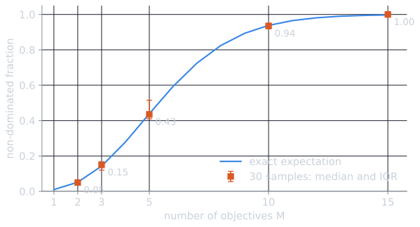
The recursion behind the exact values is short enough to derive. Let $E(n, m)$ be the expected number of non-dominated points among $n$ independent points whose $m$ coordinates are independent and continuous, so that ties have probability zero. Consider the point with the largest first coordinate. It is worse than every other point in that coordinate, so it dominates none of them, and removing it leaves the status of the other $n - 1$ points unchanged: they contribute $E(n - 1, m)$. The point itself is non-dominated exactly when no other point beats it in all of coordinates 2 to $m$, which is the event that it is non-dominated among the $n$ points projected onto those $m - 1$ coordinates. Its first coordinate plays no part in that event, so by symmetry its probability is the same for each of the $n$ points, $E(n, m - 1)/n$. Adding the two parts,
$$E(n, m) = E(n - 1, m) + \frac{E(n, m - 1)}{n}, \qquad E(n, 1) = 1, \quad E(1, m) = 1.$$
For two objectives this gives $E(n, 2) = 1 + \tfrac{1}{2} + \dots + \tfrac{1}{n}$, the harmonic number, about 5.19 for $n = 100$: a fraction of 0.052, as in the table. With one objective only the single best point is non-dominated, a fraction of 0.01; the recursion then gives 0.279 for four objectives, 0.594 for six and 0.825 for eight.
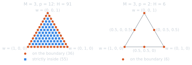
NSGA-III (Deb and Jain, 2014) keeps the NSGA-II framework and replaces the crowding distance, which is the part that fails in many dimensions. The algorithm places $H$ reference points on the unit simplex, the hyperplane on which the normalized objectives sum to 1, by the systematic method of Das and Dennis (1998). With $p$ divisions along each objective, the reference points are all vectors whose coordinates are non-negative multiples of $1/p$ summing to 1, and there are
$$H = \binom{M + p - 1}{p}$$
of them. For $M = 3$ and $p = 12$, $H = \binom{14}{12} = 91$; for $M = 5$ and $p = 6$, $H = 210$. The script enumerates these sets and confirms both counts. It also shows a limitation that Deb and Jain point out: when $p < M$, no reference point lies strictly inside the simplex. All 220 points for $M = 10$ and $p = 3$ have at least one zero coordinate, so for eight or more objectives the paper used two layers of points, a boundary layer and an inner layer.
Survivor selection proceeds as in NSGA-II until the last front $F_l$ that does not fit. Then:
- Normalize. Subtract the ideal point, the minimum of each objective over the candidates. Find an extreme point for each objective by minimizing an achievement scalarizing function, pass a hyperplane through the $M$ extreme points, and divide each objective by the hyperplane's intercept on its axis.
- Associate. Join each reference point to the origin to form a reference line, and associate each candidate with the line nearest to it in perpendicular distance.
- Count niches. For each reference point $j$, the niche count $\rho_j$ is the number of already selected members (those from the fronts before $F_l$) associated with it.
- Fill. Repeatedly take a reference point with the smallest $\rho_j$, breaking ties at random. If $\rho_j = 0$ and some member of $F_l$ is associated with it, add the one closest to its reference line; if $\rho_j \ge 1$, add a random associated member of $F_l$. Increment $\rho_j$. A reference point with no associated member in $F_l$ is excluded for the rest of the generation.
Because selection already favours sparsely populated reference directions, NSGA-III uses no tournament: parents are picked at random from the survivors. The population size is set to the smallest multiple of four greater than $H$, for example 92 for $H = 91$. Deb and Jain compared NSGA-III with two versions of MOEA/D on test problems with three to fifteen objectives, measured by the inverted generational distance to the targeted points on the front. A companion paper extended the method to constrained problems (Jain and Deb, 2014).
The lineage in one table
| Algorithm | Year | How objectives drive selection | Diversity | Elitism |
|---|---|---|---|---|
| VEGA | 1985 | One objective per subpopulation | None | No |
| MOGA | 1993 | Rank = 1 + number of dominators | Sharing in objective space | No |
| NPGA | 1994 | Domination tournaments against a sample | Niche count breaks ties | No |
| NSGA | 1994 | Non-dominated fronts, dummy fitness | Sharing within each front | No |
| SPEA | 1999 | Strength of covering archive members | Strength niching, clustering | Archive |
| PAES | 2000 | Dominance against parent and archive | Adaptive grid | Archive |
| SPEA2 | 2001 | Raw fitness from strengths | $k$-th nearest neighbour, truncation | Fixed archive |
| NSGA-II | 2002 | Non-dominated sorting | Crowding distance | Parents and offspring |
| IBEA | 2004 | Pairwise indicator values | Implicit in the indicator | Parents and offspring |
| MOEA/D | 2007 | Scalar subproblems | Spread of weight vectors | Best per subproblem |
| SMS-EMOA | 2007 | Non-dominated sorting, hypervolume | Hypervolume contribution | Steady state |
| NSGA-III | 2014 | Non-dominated sorting, reference points | Niche counts per reference line | Parents and offspring |
The years are those of the publications cited here. PAES first appeared at a 1999 conference.
Limits and open questions
Comparing these algorithms is itself a multi-objective problem. A result is a set of points, and a single number can only summarize it by adopting a preference: the hypervolume prefers some shapes of front and depends on its reference point, and distance-based measures need the true front. Rankings of algorithms can change with the indicator, as Pareto-optimal ranking of optimizers discusses. The no free lunch theorems add that no algorithm is best across all problems. The tables in the papers above are evidence about particular test problems, budgets and parameter settings, and an algorithm that leads on the ZDT problems may trail on rotated or many-objective ones.
References
- Beume, N., Naujoks, B., and Emmerich, M. (2007). SMS-EMOA: Multiobjective selection based on dominated hypervolume. European Journal of Operational Research, 181(3), 1653–1669.
- Das, I., and Dennis, J. E. (1998). Normal-boundary intersection: A new method for generating the Pareto surface in nonlinear multicriteria optimization problems. SIAM Journal on Optimization, 8(3), 631–657.
- Deb, K., and Jain, H. (2014). An evolutionary many-objective optimization algorithm using reference-point-based nondominated sorting approach, Part I: Solving problems with box constraints. IEEE Transactions on Evolutionary Computation, 18(4), 577–601.
- Deb, K., Pratap, A., Agarwal, S., and Meyarivan, T. (2002). A fast and elitist multiobjective genetic algorithm: NSGA-II. IEEE Transactions on Evolutionary Computation, 6(2), 182–197.
- Eiben, A. E., and Smith, J. E. (2015). Introduction to Evolutionary Computing, 2nd ed., chapter 12. Springer.
- Fonseca, C. M., and Fleming, P. J. (1993). Genetic algorithms for multiobjective optimization: Formulation, discussion and generalization. In Proceedings of the Fifth International Conference on Genetic Algorithms, 416–423. Morgan Kaufmann.
- Goldberg, D. E. (1989). Genetic Algorithms in Search, Optimization, and Machine Learning. Addison-Wesley.
- Horn, J., Nafpliotis, N., and Goldberg, D. E. (1994). A niched Pareto genetic algorithm for multiobjective optimization. In Proceedings of the First IEEE Conference on Evolutionary Computation, 82–87. IEEE.
- Ishibuchi, H., Tsukamoto, N., and Nojima, Y. (2008). Evolutionary many-objective optimization: A short review. In Proceedings of the 2008 IEEE Congress on Evolutionary Computation, 2419–2426. IEEE.
- Jain, H., and Deb, K. (2014). An evolutionary many-objective optimization algorithm using reference-point based nondominated sorting approach, Part II: Handling constraints and extending to an adaptive approach. IEEE Transactions on Evolutionary Computation, 18(4), 602–622.
- Knowles, J. D., and Corne, D. W. (2000). Approximating the nondominated front using the Pareto archived evolution strategy. Evolutionary Computation, 8(2), 149–172.
- Schaffer, J. D. (1985). Multiple objective optimization with vector evaluated genetic algorithms. In Proceedings of the First International Conference on Genetic Algorithms and Their Applications, 93–100. Lawrence Erlbaum.
- Srinivas, N., and Deb, K. (1994). Multiobjective optimization using nondominated sorting in genetic algorithms. Evolutionary Computation, 2(3), 221–248.
- Zhang, Q., and Li, H. (2007). MOEA/D: A multiobjective evolutionary algorithm based on decomposition. IEEE Transactions on Evolutionary Computation, 11(6), 712–731.
- Zitzler, E., Deb, K., and Thiele, L. (2000). Comparison of multiobjective evolutionary algorithms: Empirical results. Evolutionary Computation, 8(2), 173–195.
- Zitzler, E., and Künzli, S. (2004). Indicator-based selection in multiobjective search. In Parallel Problem Solving from Nature, PPSN VIII, Lecture Notes in Computer Science 3242, 832–842. Springer.
- Zitzler, E., Laumanns, M., and Thiele, L. (2001). SPEA2: Improving the Strength Pareto Evolutionary Algorithm. TIK-Report 103, Computer Engineering and Networks Laboratory (TIK), ETH Zurich.
- Zitzler, E., and Thiele, L. (1999). Multiobjective evolutionary algorithms: A comparative case study and the strength Pareto approach. IEEE Transactions on Evolutionary Computation, 3(4), 257–271.