A topic model, like a clustering, has no right answer to be checked against. Yet a model must be judged somehow: to choose the number of topics, to compare algorithms, and to decide whether the topics found are worth reading. Three kinds of evidence are used: how well the model predicts text it has not seen, how interpretable people find its topics, and automatic scores designed to stand in for those people. They do not always agree, and the disagreement is instructive.
Held-out likelihood and perplexity
A probabilistic topic model assigns a probability to any document. A good model should assign high probability to new documents from the same source, ones it was not fitted to. The standard summary is perplexity, the inverse of the geometric mean probability per word on a held-out set of documents:
$$\mathrm{perplexity} = \exp\left( - \frac{\sum_d \log p(\mathbf{w}_d)}{\sum_d N_d} \right),$$
where $\mathbf{w}_d$ is the sequence of words in held-out document $d$ and $N_d$ its length. Lower is better. A perplexity of 2,000 means the model is, on average, as uncertain about each word as if it were choosing uniformly among 2,000 equally likely words. Blei, Ng, and Jordan (2003, §7.1) used this definition to compare LDA with pLSI and simpler models.
Where the formula comes from
The formula is easier to trust once its steps are separated.
- Score the held-out text. The model's log-likelihood of the test set is $\sum_d \log p(\mathbf{w}_d)$. It is negative, and it grows more negative with every additional word, so it cannot be compared between test sets of different sizes.
- Average per word. Dividing by the number of words, $\sum_d N_d$, gives the average log-probability per word. If the model gave every word the same probability $p$, this average would be $\log p$.
- Undo the logarithm. Exponentiating the average gives the geometric mean probability per word, $\bar{p}$.
- Invert. Perplexity is $1/\bar{p}$. For a model that spreads its probability evenly over $m$ words, $\bar{p} = 1/m$ and the perplexity is exactly $m$: perplexity is the size of the uniform choice that would be equally hard to predict.
Two reference points follow. A model that ignores the data and spreads probability evenly over the vocabulary has perplexity $V$. A model that knows each word's overall frequency but nothing about documents, the unigram model, does better, and a topic model must beat it to be learning anything about documents.
A worked example
On the ten word occurrences of the five-term example of latent semantic indexing (ship twice, boat once, ocean twice, voyage three times, trip twice), scoring the same words the models were fitted to:
| Model | Log-likelihood | Perplexity |
|---|---|---|
| Uniform over the 5 words | $10 \log \tfrac{1}{5} = -16.094$ | 5.000 |
| Unigram, $P(w)$ = overall frequency | $-15.571$ | 4.745 |
| pLSA with 2 topics (best fit) | $-10.549$ | 2.872 |
| Each document its own word distribution | $-6.068$ | 1.835 |
For the unigram row, the probabilities are 0.2, 0.1, 0.2, 0.3, and 0.2, so the log-likelihood is $2 \log 0.2 + \log 0.1 + 2 \log 0.2 + 3 \log 0.3 + 2 \log 0.2 = -15.571$, and the perplexity is $e^{15.571/10} = 4.745$. The pLSA row is the fitted model of probabilistic latent semantic analysis: knowing that a document is about the sea narrows each of its words to about three equally likely choices. The last row gives each document a distribution equal to its own word frequencies, and scores better still. That is the reason perplexity must be measured on held-out text. On the training words, more parameters always look better; the last model has learned nothing that would help predict a new document. The numbers are from plsa_trace.py in tools/experiments/topics/.
Computing $p(\mathbf{w}_d)$
Computing $p(\mathbf{w}_d)$ for LDA is itself hard, since it requires averaging over all possible topic proportions for the document:
$$p(\mathbf{w}_d) = \int p(\theta \mid \alpha) \prod_{i=1}^{N_d} \sum_k \theta_k\, \phi_{k, w_{d,i}}\, d\theta.$$
The integral has no closed form, because the product of sums couples every word to every topic. Wallach, Murray, Salakhutdinov, and Mimno (2009) compared methods for estimating it and found that those in common use, the harmonic mean method most of all, were inaccurate enough to change the outcome of model comparisons. Many implementations, including scikit-learn's, report perplexity computed from a variational lower bound on the likelihood, which gives an upper bound on the true perplexity rather than the value itself. scikit-learn's bound also includes a corpus-wide term for the topic-word distributions, with consequences shown below.
A simpler alternative, used in the Reuters experiment below, is document completion: split each test document's words in two, infer the document's topic proportions $\hat{\theta}$ from the first half, and score the second half with $p(w) = \sum_k \hat{\theta}_k \phi_{k,w}$, which needs no integral. For example, the Reuters test story test/14826, on Asian exporters' fears of damage from trade friction between the United States and Japan, has 342 words after preprocessing; 171 chosen at random, among them japan eight times and trade six times, are used to infer its mixture, and the other 171 are scored.
Perplexity also measures prediction, not meaning. A model can predict words well with topics no person would find sensible.
What people think of the topics
Chang, Boyd-Graber, Gerrish, Wang, and Blei (2009) measured interpretability directly, with two tasks given to people through a crowdsourcing service:
- Word intrusion. Show the five most probable words of a topic plus one intruder, a word that is probable in another topic but not this one. If the topic is coherent, people readily spot the word that does not belong. If it is a jumble, they guess.
- Topic intrusion. Show a document's title and opening, three topics prominent in it, and one that is not. People who can spot the intruding topic find the document's assigned topics meaningful.
Building and scoring an item
The construction is precise (Chang and colleagues, 2009, §3). For word intrusion, the intruder is drawn from words with low probability in the topic, so that it is unlikely to belong to the same subject, but high probability in some other topic, so that it cannot be rejected merely for being rare. The six words are shuffled. For the Reuters "Oil markets" topic of the LDA article, whose top five words are oil, opec, bpd, crude, and gulf, a valid intruder is dividend: it is in the bottom half of the oil topic's words and among the ten most probable words of the dividend and stock-split topics. A reader shown
crude, dividend, gulf, oil, bpd, opec
picks dividend at once, which is evidence that the other five form a subject. For the incoherent topic whose top words are department, dutch, guilders, credit, and hughes, no such choice is obvious.
Each item is shown to several people (eight in the original study). If $\omega$ is the true intruder and $i_s$ the word chosen by person $s$, the topic's model precision is the fraction who found it:
$$\mathrm{MP} = \frac{1}{S} \sum_{s=1}^{S} \mathbf{1}(i_s = \omega).$$
If seven of eight readers chose dividend, the oil topic would score $7/8 = 0.875$; a topic where readers guess at random among six words would score about $1/6$. Topic intrusion is scored by the topic log odds, the average over people of $\log \hat{\theta}_{d, j^*} - \log \hat{\theta}_{d, j_s}$, where $j^*$ is the true intruding topic and $j_s$ the one person $s$ chose. It is 0 when everyone finds the intruder, and more negative the more probable the topics people mistook for it (Chang and colleagues, 2009, eqs. 1 and 2).
What they found
They fitted pLSI, LDA, and the correlated topic model with 50, 100, and 150 topics to New York Times and Wikipedia articles. Their central finding was that held-out likelihood did not predict interpretability and could run against it. The correlated topic model had the best predictive likelihood, but its topics fared worst with people, and plots of the human scores against likelihood showed no gain, and often a loss, as likelihood improved. A model tuned only for perplexity is not tuned for what most users of topic models want.
Coherence measures
Human evaluation is slow and expensive, so automatic coherence measures were developed to approximate it. Most score a topic by how often its top words occur together in documents, on the reasoning that a coherent topic's words belong to the same subject and so co-occur.
- UMass coherence (Mimno, Wallach, Talley, Leenders, and McCallum, 2011) uses co-document frequencies from the collection the model was fitted to, $\sum \log \frac{D(w_i, w_j) + 1}{D(w_j)}$ over ordered pairs of top words with $w_j$ ranked above $w_i$, where $D$ counts documents. The measure is asymmetric.
- PMI coherence (Newman, Lau, Grieser, and Baldwin, 2010) averages the pointwise mutual information between pairs of top words, estimated from a large external corpus such as Wikipedia.
- NPMI coherence normalizes each pair's PMI by $-\log P(w_i, w_j)$, so it ranges from −1, for words that never appear together, through 0, for independence, to 1, for words that always appear together (Bouma, 2009). Lau, Newman, and Baldwin (2014) found it among the measures that best matched human judgments.
For a topic with top words $w_1, \dots, w_n$, NPMI coherence is the average over pairs:
$$\mathrm{NPMI}(w_i, w_j) = \frac{\log \dfrac{P(w_i, w_j)}{P(w_i)\,P(w_j)}}{-\log P(w_i, w_j)}.$$
Each piece has a reading. The ratio inside the logarithm compares how often the two words share a document with how often they would if they were independent; its logarithm, the PMI, is positive for words that attract each other. PMI has no fixed scale, since rare pairs can reach large values, so NPMI divides by $-\log P(w_i, w_j)$, the largest value PMI can take for a pair with that joint probability (reached when each word appears only with the other). In the UMass score, $(D(w_i, w_j) + 1) / D(w_j)$ is an estimate of the conditional probability of $w_i$ given $w_j$, the share of documents with the higher-ranked word that also contain the lower-ranked one, with 1 added so that a pair that never co-occurs gives a finite logarithm.
Two topics scored by hand
Take the top five words of two topics from the twenty-topic Reuters model in the LDA article, with probabilities estimated from the 7,769 training stories by counting the stories that contain each word and each pair (natural logarithms throughout). First, the "Energy production" topic, whose document frequencies are oil 730, gas 275, energy 237, reserves 274, and production 515:
| Pair | $D(w_i)$, $D(w_j)$ | $D(w_i, w_j)$ | UMass term | PMI | NPMI |
|---|---|---|---|---|---|
| oil, gas | 730, 275 | 207 | −1.256 | 2.081 | 0.574 |
| oil, energy | 730, 237 | 147 | −1.596 | 1.887 | 0.476 |
| gas, energy | 275, 237 | 84 | −1.174 | 2.304 | 0.509 |
| oil, reserves | 730, 274 | 74 | −2.276 | 1.056 | 0.227 |
| gas, reserves | 275, 274 | 51 | −1.666 | 1.660 | 0.330 |
| energy, reserves | 237, 274 | 22 | −2.333 | 0.968 | 0.165 |
| oil, production | 730, 515 | 169 | −1.457 | 1.251 | 0.327 |
| gas, production | 275, 515 | 74 | −1.299 | 1.401 | 0.301 |
| energy, production | 237, 515 | 76 | −1.124 | 1.576 | 0.341 |
| reserves, production | 274, 515 | 49 | −1.701 | 0.992 | 0.196 |
In each pair the first word is the higher-ranked one, whose frequency goes in the UMass denominator. For the first row: $P(\text{oil}) = 730/7769 = 0.0940$, $P(\text{gas}) = 275/7769 = 0.0354$, and $P(\text{oil}, \text{gas}) = 207/7769 = 0.0266$. The words share a document $0.0266 / (0.0940 \times 0.0354) = 8.0$ times as often as independence would predict, so the PMI is $\log 8.0 = 2.081$, and dividing by $-\log 0.0266 = 3.625$ gives NPMI 0.574. The UMass term is $\log(208/730) = -1.256$. Over the ten pairs, UMass coherence is the sum, $-15.88$, and NPMI coherence the mean, $0.344$.
Second, the incoherent topic, with top words department (430 stories), dutch (97), guilders (37), credit (342), and hughes (19). Four of its ten pairs never occur in the same story: department with guilders, and hughes with dutch, guilders, and credit. Each of those gets NPMI −1 and a UMass term of $\log(1/D(w_j))$, as low as $\log(1/430) = -6.06$. Only dutch and guilders go together (29 shared stories, NPMI 0.740). Its UMass coherence is $-37.50$ and its NPMI coherence $-0.282$. Both measures separate the two topics by a wide margin, and they agree on the order, though the UMass score has no fixed scale on which to say how good $-15.88$ is.
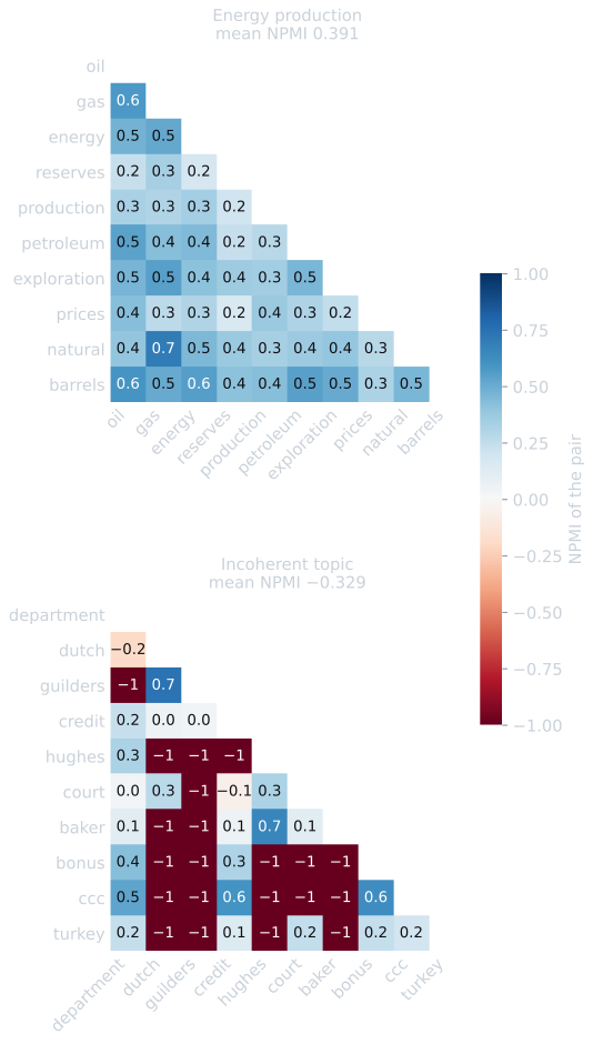
With all ten top words, as in the rest of this article, the two topics score 0.391 and −0.329. The pair matrix shows why the second is junk in a way the single number does not: it is not a weak subject but a few strong word pairs, such as dutch and guilders, hughes and baker, and bonus and ccc, that almost never share a story with each other.
Coherence measures are proxies too. Hoyle and colleagues (2021) found that automatic coherence had rarely been validated for newer neural topic models and could disagree with human ratings of them, and recommended that claims of better topics be checked with people.
On Reuters
The LDA model of Reuters was fitted with five values of $K$ to the 7,769 training stories, and evaluated on the 3,019 test stories. Held-out perplexity was measured by document completion (Rosen-Zvi, Griffiths, Steyvers, and Smyth, 2004; Wallach, Murray, Salakhutdinov, and Mimno, 2009): each test story's words were split in half at random, the story's topic proportions were inferred from the first half, and the second half, 78,587 words in all from the 3,017 stories long enough to split, was scored with the fitted topics. The inferred proportions serve as a point estimate, a simpler approximation than the estimators Wallach and colleagues recommend, but one that scores only the held-out words. Coherence is the average NPMI of each topic's ten most probable words, with probabilities estimated from document co-occurrence in the training stories.
| Topics $K$ | Held-out perplexity (document completion) | scikit-learn's reported test perplexity | Mean NPMI |
|---|---|---|---|
| 5 | 1,517 | 2,158 | 0.203 |
| 10 | 1,339 | 2,240 | 0.242 |
| 20 | 1,174 | 2,376 | 0.251 |
| 40 | 1,096 | 2,916 | 0.208 |
| 80 | 1,066 | 4,319 | 0.122 |
For scale, the same 78,587 held-out words have perplexity 6,855 under the uniform distribution over the vocabulary and 2,238 under the unigram distribution of the training stories (with 1 added to each count). Even five topics cut the unigram perplexity by a third; twenty cut it nearly in half.
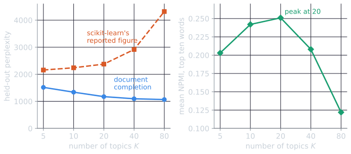
Three things stand out:
- Held-out perplexity improved at every step, quickly up to 20 topics and slowly after that. More topics let the model predict new stories' words better, with diminishing returns.
- scikit-learn's own figure pointed the opposite way. Its
perplexitymethod uses the variational bound on the likelihood of the whole model, which includes a term for the topic-word distributions themselves. That term does not depend on the documents scored, grows with the number of topics, and is divided by the number of words in the test set, so the reported value rises with $K$ for reasons that have nothing to do with prediction. Read naively, it would suggest that five topics is best and that the model overfits. From 10 topics on it is no better than the unigram model's 2,238, a model with no topics at all (scikit-learn scores the whole test stories rather than their second halves, so the comparison is approximate), while the document-completion measure puts every one of these models well below it. The document-completion measure shows neither problem. - Coherence peaked at 20 topics. With five or ten topics, each topic must cover several subjects, and its top words co-occur less. With 40 or 80, topics fragment into narrow, sometimes accidental word groups.
So the measures disagree much as Chang and colleagues found, with coherence standing in for human judgment. Prediction kept improving as topics were added, while coherence fell after 20. Five topics are too few for a collection with dozens of subjects, so each must combine several. Twenty topics give the readable list in the LDA article. For exploring a collection, which is what most topic models are used for, coherence and inspection pointed to the more useful choice. The episode also shows why an evaluation number should be understood before it is trusted: the convenient figure from the library would have led to the wrong conclusion.
Scoring individual topics
Coherence is also useful topic by topic, to flag ones not worth reading. Apart from one topic, scores among the twenty ranged from 0.391 for energy production (oil, gas, energy, reserves, production) down to 0.076 for the mixed topic of metals and European currencies. One topic scored −0.329: department, dutch, guilders, credit, hughes, court, baker, bonus, ccc, turkey. These words rarely occur in the same stories, and no person would call them a subject. Coherence flagged exactly the topic that inspection does.
The same measure applied to LSI on the same stories, scoring the ten terms with the largest positive weight in each of 20 dimensions, gave a mean of 0.097, against 0.251 for LDA with 20 topics. LSI's dimensions are contrasts between groups of words, not groups of words in their own right, so their top terms are not meant to form a subject, and the score reflects that.
Choosing the number of topics
No method settles $K$. In practice it is chosen by:
- fitting several values and comparing coherence, held-out likelihood, or both, while expecting them to disagree;
- reading the topics, since a model with a few junk topics or with obviously merged subjects needs a different $K$;
- checking stability, refitting with different random starts and seeing whether the same topics reappear, since topics that appear only in some runs should not be trusted;
- letting the purpose decide, since a browsing interface needs few broad topics and a fine-grained analysis many narrow ones.
Nonparametric models, described in topic models beyond LDA, infer the number of topics from the data, though they have parameters of their own that influence how many they find.
The experiments are reuters_lda.py, reuters_perplexity.py, reuters_perplexity_baselines.py, and reuters_coherence_hand.py in tools/experiments/topics/ in the site repository, and the figures are drawn by tools/figures/evaluating-topic-models.py.
References
- Blei, D. M., Ng, A. Y., and Jordan, M. I. (2003). Latent Dirichlet allocation. Journal of Machine Learning Research, 3, 993–1022.
- Bouma, G. (2009). Normalized (pointwise) mutual information in collocation extraction. In Proceedings of the Biennial GSCL Conference, 31–40.
- Chang, J., Boyd-Graber, J., Gerrish, S., Wang, C., and Blei, D. M. (2009). Reading tea leaves: How humans interpret topic models. In Advances in Neural Information Processing Systems 22 (NIPS 2009), 288–296.
- Hoyle, A., Goel, P., Hian-Cheong, A., Peskov, D., Boyd-Graber, J., and Resnik, P. (2021). Is automated topic model evaluation broken? The incoherence of coherence. In Advances in Neural Information Processing Systems 34 (NeurIPS 2021).
- Lau, J. H., Newman, D., and Baldwin, T. (2014). Machine reading tea leaves: Automatically evaluating topic coherence and topic model quality. In Proceedings of EACL 2014, 530–539.
- Mimno, D., Wallach, H. M., Talley, E., Leenders, M., and McCallum, A. (2011). Optimizing semantic coherence in topic models. In Proceedings of EMNLP 2011, 262–272.
- Newman, D., Lau, J. H., Grieser, K., and Baldwin, T. (2010). Automatic evaluation of topic coherence. In Proceedings of NAACL-HLT 2010, 100–108.
- Rosen-Zvi, M., Griffiths, T., Steyvers, M., and Smyth, P. (2004). The author-topic model for authors and documents. In Proceedings of UAI 2004, 487–494.
- Wallach, H. M., Murray, I., Salakhutdinov, R., and Mimno, D. (2009). Evaluation methods for topic models. In Proceedings of ICML 2009, 1105–1112.