A classifier can be checked against the right answers. A clustering, by definition, has none: it was asked to find groups no one specified. Judging one therefore means deciding what "good" should mean, and the main choices give different answers. This article describes the two families of criteria, defines the standard external measures, and works through each on the example in Manning, Raghavan, and Schütze (2008, §16.3), whose numbers were recomputed for this article. It then tests the measures on clusterings that should score badly, which shows what each one rewards.
Internal and external criteria
An internal criterion scores a clustering by its own geometry: how similar documents are within clusters and how dissimilar across them. The residual sum of squares that K-means minimizes is one. Internal criteria need no labels, but a high score does not mean the clustering is useful. A clustering can be tight and well separated along a dimension no one cares about. Internal criteria also favor whichever algorithm optimizes them, so they cannot fairly compare algorithms.
An external criterion compares the clustering with a set of classes chosen by people, such as the categories of a labeled collection. This measures what usually matters, whether the clusters correspond to distinctions people make, but it requires labels, and it assumes that the given classes are the right answer. As K-means in practice shows on Reuters, an algorithm can find coherent groups that simply differ from the editors' categories.
A third option, the most direct, is to measure the clustering's effect on a task, such as how much faster users find relevant documents when results are clustered. This is the most informative and the most expensive.
The rest of this article covers external criteria. Only the grouping given by the classes matters, not their names: an external measure compares two partitions of the same documents.
The worked example
Seventeen documents from three classes, which the textbook draws as x, o, and ◇, are grouped into three clusters:
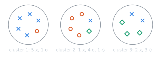
As a contingency table, with one row per cluster, one column per class, and the totals on the margins:
| Cluster | x | o | ◇ | Cluster size |
|---|---|---|---|---|
| 1 | 5 | 1 | 0 | 6 |
| 2 | 1 | 4 | 1 | 6 |
| 3 | 2 | 0 | 3 | 5 |
| Class size | 8 | 5 | 4 | 17 |
Every measure below is a function of this table alone. Write $n_{kj}$ for the entry in row $k$ and column $j$, $n_k$ for the size of cluster $k$, $n_j$ for the size of class $j$, and $N = 17$ for the total.
Purity
Purity assigns each cluster to its most frequent class and counts the fraction of documents that match their cluster's class:
$$\mathrm{purity}(\Omega, C) = \frac{1}{N} \sum_k \max_j \lvert \omega_k \cap c_j \rvert,$$
where $\Omega = \{\omega_1, \dots, \omega_K\}$ are the clusters and $C = \{c_1, \dots, c_J\}$ the classes. In the example the row maxima are 5, 4, and 3, so purity is $12/17 \approx 0.71$. It is the accuracy a classifier would have if it labeled every document with its cluster's majority class.
Purity is easy to understand and has one serious flaw: it rewards many clusters. Splitting a cluster never lowers purity, because the majority count of the whole is at most the sum of the majority counts of the parts: $\max_j (a_j + b_j) \le \max_j a_j + \max_j b_j$. With one document per cluster, every cluster is pure, and purity is 1. Purity can only compare clusterings with the same number of clusters.
Normalized mutual information
Mutual information measures how much a document's cluster reveals about its class:
$$I(\Omega; C) = \sum_k \sum_j \frac{n_{kj}}{N} \log \frac{N\, n_{kj}}{n_k\, n_j}.$$
Each term compares how often cluster $k$ and class $j$ occur together, $n_{kj}/N$, with how often they would if clusters and classes were independent, $(n_k/N)(n_j/N)$. Where they co-occur more than independence predicts, the logarithm is positive. It is the same quantity used for feature selection, here measured between clusters and classes rather than terms and classes.
In the example, with natural logarithms and rounded to four decimals, the seven nonzero cells contribute:
| Cell | $n_{kj}/N$ | $\log \dfrac{N n_{kj}}{n_k n_j}$ | Term |
|---|---|---|---|
| cluster 1, x | 5/17 | ln(85/48) = 0.5715 | 0.1681 |
| cluster 1, o | 1/17 | ln(17/30) = −0.5680 | −0.0334 |
| cluster 2, x | 1/17 | ln(17/48) = −1.0380 | −0.0611 |
| cluster 2, o | 4/17 | ln(68/30) = 0.8183 | 0.1925 |
| cluster 2, ◇ | 1/17 | ln(17/24) = −0.3448 | −0.0203 |
| cluster 3, x | 2/17 | ln(34/40) = −0.1625 | −0.0191 |
| cluster 3, ◇ | 3/17 | ln(51/20) = 0.9361 | 0.1652 |
The majority cells add information and the stray documents subtract a little, for a total of $I = 0.3919$ nats.
Like purity, mutual information reaches its maximum with one document per cluster: knowing a document's singleton cluster tells everything about its class, so $I$ equals the entropy of the classes. Normalized mutual information divides by the average entropy of the clusters and the classes:
$$\mathrm{NMI}(\Omega, C) = \frac{I(\Omega; C)}{[H(\Omega) + H(C)]/2}, \qquad H(\Omega) = -\sum_k \frac{n_k}{N} \log \frac{n_k}{N}.$$
The entropies in the example are
$$H(\Omega) = -2 \cdot \tfrac{6}{17} \ln \tfrac{6}{17} - \tfrac{5}{17} \ln \tfrac{5}{17} = 1.0951, \qquad H(C) = -\tfrac{8}{17} \ln \tfrac{8}{17} - \tfrac{5}{17} \ln \tfrac{5}{17} - \tfrac{4}{17} \ln \tfrac{4}{17} = 1.0551,$$
so NMI is $0.3919 / 1.0751 = 0.365$, the textbook's 0.36. The base of the logarithm cancels in the ratio.
The entropy $H(\Omega)$ grows with the number of clusters, reaching $\log N$ for singletons, so the denominator penalizes fragmentation. NMI ranges from 0, when the clusters carry no information about the classes, to 1, when they match exactly. Other normalizations are also used, such as the geometric mean of the two entropies (Strehl and Ghosh, 2002), so NMI values from different sources are not always comparable. (In this example the two normalizations agree to three decimals.)
The Rand index
The Rand index (Rand, 1971) views clustering as a series of decisions about pairs of documents. Each of the $\binom{N}{2}$ pairs is either put in the same cluster or not, and either belongs to the same class or not:
| Same class | Different classes | |
|---|---|---|
| Same cluster | true positive (TP) | false positive (FP) |
| Different clusters | false negative (FN) | true negative (TN) |
The Rand index is the fraction of pair decisions that are correct:
$$\mathrm{RI} = \frac{TP + TN}{TP + FP + FN + TN}.$$
The four counts come from the contingency table by counting pairs, $\binom{n}{2} = n(n-1)/2$ for a group of $n$:
- All pairs. The 17 documents form $\binom{17}{2} = 136$ pairs.
- Same cluster (TP + FP): pairs inside a row's total, $\binom{6}{2} + \binom{6}{2} + \binom{5}{2} = 15 + 15 + 10 = 40$.
- Same cluster and same class (TP): pairs inside a single cell, $\binom{5}{2} + \binom{4}{2} + \binom{3}{2} + \binom{2}{2} = 10 + 6 + 3 + 1 = 20$. Cells of 1 contribute no pairs. So FP $= 40 - 20 = 20$.
- Same class (TP + FN): pairs inside a column's total, $\binom{8}{2} + \binom{5}{2} + \binom{4}{2} = 28 + 10 + 6 = 44$. So FN $= 44 - 20 = 24$.
- The rest are true negatives: TN $= 136 - 20 - 20 - 24 = 72$.
The Rand index is $(20 + 72)/136 \approx 0.68$.
Because most pairs in a collection with several classes belong to different classes, true negatives dominate, and the Rand index tends to be high even for poor clusterings. The next sections make this concrete.
The adjusted Rand index
A natural fix is to ask how many true positives a clustering has beyond what chance would give. Keep the cluster sizes and class sizes fixed, and imagine the documents' classes shuffled at random among them. Each of the 40 same-cluster pairs is then a same-class pair with probability equal to the overall fraction of same-class pairs, $44/136$. The expected number of true positives is therefore
$$E[TP] = \frac{(TP + FP)(TP + FN)}{\binom{N}{2}} = \frac{40 \times 44}{136} = 12.94.$$
The example's 20 true positives exceed that by 7.06. To put this on a scale from 0 to 1, divide by the largest possible excess. TP cannot exceed either the 40 same-cluster pairs or the 44 same-class pairs, and the usual convention takes the maximum as their average, 42. The adjusted Rand index (Hubert and Arabie, 1985) is then
$$\mathrm{ARI} = \frac{TP - E[TP]}{\tfrac{1}{2}\left[(TP + FP) + (TP + FN)\right] - E[TP]} = \frac{20 - 12.94}{42 - 12.94} = 0.243.$$
Chance agreement scores about 0, perfect agreement 1, and a clustering worse than chance scores below 0. The value 0.243 is the same that scikit-learn's implementation returns for this table. It is much lower than the Rand index of 0.68 because most of the Rand index's credit here was for the 72 true negatives, which a random clustering of the same sizes would also earn in large numbers.
The F measure
The pair counts also give precision and recall: $P = TP/(TP + FP)$, the fraction of same-cluster pairs that are same-class, and $R = TP/(TP + FN)$, the fraction of same-class pairs that were put together. In the example, $P = 20/40 = 0.5$ and $R = 20/44 \approx 0.455$, so
$$F_1 = \frac{2PR}{P + R} = \frac{2 \times 0.5 \times 0.455}{0.955} \approx 0.48.$$
The F measure lets an evaluator weigh the two kinds of error. Separating similar documents is a false negative; grouping dissimilar ones is a false positive. The general form is $F_\beta = (\beta^2 + 1)PR/(\beta^2 P + R)$, and setting $\beta > 1$ weights recall more heavily, which penalizes false negatives more. With $\beta = 5$ the example scores $F_5 = 26 \times 0.5 \times 0.455 / (25 \times 0.5 + 0.455) \approx 0.46$, close to its recall.
Degenerate and random clusterings
A good way to understand a measure is to feed it clusterings that should score badly. Three are useful for the example's seventeen documents: every document in its own cluster (singletons), all documents in one cluster, and random clusterings that keep the three cluster sizes 6, 6 and 5 but assign documents to them at random. The random row gives the median over 30 seeded shuffles. Values are rounded to three decimals.
| Clustering | Purity | NMI | RI | ARI |
|---|---|---|---|---|
| The example | 0.706 | 0.365 | 0.676 | 0.243 |
| Singletons | 1 | 0.543 | 0.676 | 0 |
| One cluster | 0.471 | 0 | 0.324 | 0 |
| Random, same sizes | 0.529 | 0.114 | 0.574 | 0.002 |
The interquartile ranges of the random clusterings are 0.471 to 0.632 for purity, 0.050 to 0.228 for NMI, 0.544 to 0.618 for the Rand index, and −0.067 to 0.105 for the ARI. The F measures of the first three clusterings:
| Clustering | $F_1$ | $F_5$ |
|---|---|---|
| The example | 0.476 | 0.456 |
| Singletons | 0 | 0 |
| One cluster | 0.489 | 0.926 |
Each measure has a blind spot:
- Purity gives the singletons a perfect 1, as shown above.
- NMI also prefers the singletons, 0.543, to the actual clustering, 0.365. The normalization reduces the reward for fragmentation but does not remove it: for singletons, NMI is $2H(C)/(H(C) + \log N)$, which falls toward 0 only as $N$ grows. With 17 documents and three classes it is still large. Random clusterings also score above 0, a median of 0.114.
- The Rand index gives the singletons exactly the same score as the example, 92/136 = 0.676. The singletons get every one of the 92 different-class pairs right by never putting anything together, and the example earns the same 92 correct decisions a different way, 20 true positives plus 72 true negatives.
- The adjusted Rand index gives both degenerate clusterings 0 and random clusterings about 0, as it was designed to, while keeping a clear positive score for the example.
- $F_5$, which weights recall heavily, gives its best score of the table, 0.926, to the single cluster, because putting everything together finds every same-class pair. A heavily recall-weighted F measure rewards lumping in the same way that purity rewards splitting. Even $F_1$ rates the single cluster, 0.489, slightly above the example, 0.476.
None of the measures is wrong; each answers a narrower question than "is this a good clustering". Purity and $F_\beta$ with large $\beta$ should only compare clusterings with the same number of clusters. Measures adjusted for chance, such as the ARI, are the safest when the number of clusters differs.
The measures on Reuters
The measures disagree in useful ways on real data as well. On the six-category Reuters collection in K-means in practice, ten random-start K-means runs with $K = 6$ gave purity from 0.703 to 0.804 and NMI from 0.372 to 0.496, while the Rand index stayed between 0.659 and 0.721. The lowest-RSS clustering found with k-means++ split the large earn category into four clusters and put nearly all of three small categories, and three quarters of a fourth, into one. Its purity was 0.745, because most clusters are dominated by one category, while its NMI was only 0.382, because the clusters say little about which of the small categories a story belongs to.
The blind spots found on seventeen documents show up at scale when the number of clusters varies. The same collection was clustered with $K$ from 2 to 50, with 30 k-means++ runs for each $K$, and every clustering was also compared with a random clustering of the same cluster sizes:
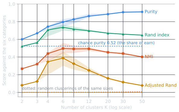
| $K$ | Purity | NMI | Rand index | Adjusted Rand |
|---|---|---|---|---|
| 2 | 0.601 | 0.268 | 0.521 | 0.081 |
| 4 | 0.744 | 0.439 | 0.706 | 0.347 |
| 6 | 0.796 | 0.496 | 0.736 | 0.388 |
| 12 | 0.863 | 0.493 | 0.697 | 0.249 |
| 20 | 0.885 | 0.454 | 0.670 | 0.160 |
| 50 | 0.910 | 0.402 | 0.647 | 0.078 |
(Medians of 30 runs, rounded to three decimals.) Purity rises at every step, from 0.60 to 0.91, because more clusters can each be dominated by one category; by $K = 50$ the clustering has carved the collection into small, nearly pure pieces and purity says it is the best yet. The adjusted Rand index says the opposite: it peaks at $K = 6$ and falls to 0.08 at $K = 50$, because fifty clusters separate most pairs of stories that share a category. NMI sits between them, nearly flat from 6 to 12 clusters and falling slowly after. Its normalization does what the textbook says on a collection of this size: assigning each of the 7,487 stories its own cluster would score an NMI of only 0.24, far below the real clusterings.
The chance baselines explain the starting points of the curves. A random clustering's purity is about 0.52 for every $K$, because the earn category holds 52 percent of the stories and is the majority in almost every random cluster. Random NMI rises slightly with $K$, from 0.0002 to 0.007, and random ARI stays at 0. On a collection this large, chance NMI is negligible; on the seventeen documents above it was not.
The other caution is the classes themselves. A low external score can mean the algorithm failed, or that it found a different and equally sensible structure. Reading the contingency table, and the terms that characterize each cluster, is usually more informative than any single number.
Summary
| Measure | Range | Rewards more clusters? | Example value |
|---|---|---|---|
| Purity | 0 to 1 | Yes, reaching 1 at one document per cluster | 0.71 |
| NMI | 0 to 1 | Less than purity: the normalization penalizes fragmentation, but singletons can still outscore a sensible clustering | 0.36 |
| Rand index | 0 to 1 | Not directly, but inflated by the many true negatives | 0.68 |
| Adjusted Rand index | about 0 for chance, up to 1 | No: chance and degenerate clusterings score about 0 | 0.24 |
| F measure | 0 to 1 | Adjustable through β; large β rewards fewer clusters | $F_1$ 0.48, $F_5$ 0.46 |
The scripts that recompute the example are tools/experiments/clustering/textbook_eval.py and tools/experiments/clustering/eval_worked.py in the site repository; the Reuters measures come from the Reuters scripts in the same folder.
References
- Hubert, L., and Arabie, P. (1985). Comparing partitions. Journal of Classification, 2(1), 193–218.
- Manning, C. D., Raghavan, P., and Schütze, H. (2008). Introduction to Information Retrieval, section 16.3. Cambridge University Press.
- Rand, W. M. (1971). Objective criteria for the evaluation of clustering methods. Journal of the American Statistical Association, 66(336), 846–850.
- Strehl, A., and Ghosh, J. (2002). Cluster ensembles: A knowledge reuse framework for combining multiple partitions. Journal of Machine Learning Research, 3, 583–617.