Latent Dirichlet allocation (LDA), introduced by Blei, Ng, and Jordan (2003), is the most widely used topic model. It keeps the picture of pLSA, topics as distributions over words and documents as mixtures of topics, and adds the missing piece: an account of where each document's mixture comes from. That makes LDA a complete generative model of documents, with a fixed number of parameters however large the collection, and a probability for any document, including ones it has never seen.
This article states the model, explains the Dirichlet distribution it is named for, derives the collapsed Gibbs sampler step by step and traces it on the six-document example used throughout the topic, and then fits twenty topics to Reuters.
The generative story
LDA imagines that a collection was produced by a random process. With $K$ topics and a vocabulary of $V$ words (the pLSA article calls the vocabulary size $M$):
- For each topic $k$, draw a distribution over words $\phi_k \sim \mathrm{Dirichlet}(\beta)$.
- For each document $d$:
- Draw its topic proportions $\theta_d \sim \mathrm{Dirichlet}(\alpha)$.
- For each word position $i$ in the document:
- Draw a topic $z_{d,i}$ from the proportions $\theta_d$.
- Draw the word $w_{d,i}$ from that topic's distribution $\phi_{z_{d,i}}$.
No one believes documents are written this way. Word order is ignored, and topics do not choose words independently. The story is a device: if documents had been produced like this, the topics and proportions that best explain the observed words are the ones worth finding. Only the words $w$ are observed. The topics $\phi$, the proportions $\theta$, and the assignments $z$ are all latent, and fitting LDA means inferring them.
The difference from pLSA is step 2.1. In pLSA, each document's proportions are free parameters. In LDA they are random variables drawn from one shared distribution, controlled by a single parameter $\alpha$. The notation follows the smoothed version of the model (Blei, Ng, and Jordan, 2003, §5.4) and Griffiths and Steyvers (2004). In Blei, Ng, and Jordan's paper, $\beta$ names the topic-word matrix itself, and in the smoothed version the prior on it is $\eta$, as in scikit-learn. The model's parameters are just $\alpha$ and $\beta$, and every document, seen or unseen, gets a probability by averaging over the proportions it might have had.
Plate notation
The same story is usually drawn as a graphical model, in which circles are random variables, arrows point from a variable to the ones drawn from it, and a rectangle, a plate, means "repeat what is inside" the number of times written in its corner.
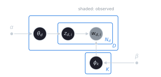
Multiplying one factor per circle, each conditioned on its parents, gives the joint probability of everything in the picture:
$$p(\phi, \theta, z, w \mid \alpha, \beta) = \prod_{k=1}^{K} p(\phi_k \mid \beta) \prod_{d=1}^{D} \left( p(\theta_d \mid \alpha) \prod_{i=1}^{N_d} \theta_{d, z_{d,i}}\, \phi_{z_{d,i}, w_{d,i}} \right).$$
Everything in inference starts from this product. pLSA's diagram would have no $\alpha$ node, and $\theta_d$ would be a fixed parameter rather than a circle.
The Dirichlet distribution
Topic proportions and topics are both probability vectors, lists of nonnegative numbers summing to 1. The Dirichlet distribution is a distribution over such vectors. In the symmetric form used here, with $K$ components and concentration parameter $\alpha$, its density is
$$p(\theta \mid \alpha) = \frac{\Gamma(K\alpha)}{\Gamma(\alpha)^K} \prod_{k=1}^{K} \theta_k^{\alpha - 1}.$$
The fraction in front only makes the density integrate to 1. The shape comes from the product: each $\theta_k^{\alpha - 1}$ is large near $\theta_k = 0$ when $\alpha < 1$ (a negative power), flat when $\alpha = 1$, and small near 0 when $\alpha > 1$. In the general, asymmetric form each component has its own $\alpha_k$, the fraction becomes $\Gamma(\sum_k \alpha_k) / \prod_k \Gamma(\alpha_k)$, and component $k$ has mean $\alpha_k / \sum_j \alpha_j$.
With three components the vectors are points in a triangle, and the effect of $\alpha$ can be seen:
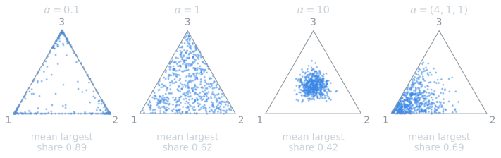
Every component of a symmetric Dirichlet has the same expected value, $1/K$. What $\alpha$ controls is how far a typical draw strays from that average:
| $\alpha$, with $K = 20$ | Average size of the largest component |
|---|---|
| 0.05 | 0.65 |
| 0.5 | 0.25 |
| 1 | 0.18 |
| 10 | 0.08 |
With $\alpha$ below 1, draws are sparse, concentrated on a few components. With $\alpha = 0.05$, a typical document puts about two-thirds of its weight on one topic. With $\alpha$ well above 1, draws are close to uniform, and every document is a little of everything. Small values suit text, since most documents are about a few things. Settings in practice vary: Griffiths and Steyvers (2004) used $\alpha = 50/K$, which is above 1 for fewer than 50 topics and so favors broader mixtures, with $\beta = 0.1$, while scikit-learn's defaults are $1/K$ for both. A small $\beta$ makes each topic concentrate on a modest set of words. (The table's values come from 10,000 draws for each setting; dirichlet_demo.py in tools/experiments/topics/. The figure's 600 draws per panel are drawn by tools/figures/latent-dirichlet-allocation.py.)
Conjugacy and pseudo-counts
The Dirichlet is also the conjugate prior of the multinomial: after observing counts, the posterior is again Dirichlet, with the counts added to the parameters. The reason is visible in the formulas. If a document's topic assignments include $n_k$ words from topic $k$, their probability given $\theta$ is $\prod_k \theta_k^{n_k}$. Multiplying by the prior $\prod_k \theta_k^{\alpha - 1}$ gives $\prod_k \theta_k^{n_k + \alpha - 1}$, which is the shape of a Dirichlet with parameters $n_k + \alpha$. For example, a two-topic document with prior $\alpha = 0.1$ that has two words assigned to topic 1 and one to topic 2 has posterior $\mathrm{Dirichlet}(2.1, 1.1)$, whose mean is $(2.1/3.2,\ 1.1/3.2) = (0.656, 0.344)$, against the raw proportions $(0.667, 0.333)$.
That property is what makes the inference below tractable, and it gives $\alpha$ and $\beta$ an interpretation as pseudo-counts, imaginary observations added to every topic in every document and to every word in every topic, the same idea as the add-one smoothing of Naive Bayes. The normalizing constant of the Dirichlet will be needed below. Write
$$B(a_1, \dots, a_K) = \frac{\prod_k \Gamma(a_k)}{\Gamma\!\left(\sum_k a_k\right)},$$
so that the density is $\prod_k \theta_k^{a_k - 1} / B(a)$, and therefore $\int \prod_k \theta_k^{a_k - 1}\, d\theta = B(a)$ over the simplex.
Inference
Given the documents, the goal is the posterior distribution of the latent variables, $p(\theta, \phi, z \mid w)$. Its normalizing constant sums over every possible assignment of topics to every word in the collection, $K^n$ assignments for $n$ word occurrences, and cannot be computed exactly. For the 450,424 word occurrences of the Reuters training set below with $K = 20$, that is $20^{450{,}424}$ assignments. Two families of approximation are standard.
Collapsed Gibbs sampling
Griffiths and Steyvers (2004) observed that $\theta$ and $\phi$ can be integrated out, thanks to conjugacy, leaving only the topic assignments $z$. Gibbs sampling then visits each word occurrence in turn and resamples its topic from its conditional distribution given all the other assignments:
$$P(z_i = k \mid z_{-i}, w) \propto \left(n_{d,k}^{-i} + \alpha\right) \frac{n_{k,w_i}^{-i} + \beta}{n_{k}^{-i} + V\beta}.$$
Here $n_{d,k}^{-i}$ is the number of other words in document $d$ assigned to topic $k$, $n_{k,w_i}^{-i}$ the number of times word $w_i$ is assigned to topic $k$ across the collection, and $n_k^{-i}$ the total number of words assigned to topic $k$, all excluding the current word. The two factors read naturally: a word is likely to be assigned to a topic that is common in its document and that often produces this word. Each sweep through the collection costs time proportional to the number of word occurrences times $K$. After many sweeps, the assignments are samples from the posterior, and estimates of the topics and proportions follow from the counts:
$$\hat{\phi}_{k,w} = \frac{n_{k,w} + \beta}{n_k + V\beta}, \qquad \hat{\theta}_{d,k} = \frac{n_{d,k} + \alpha}{n_d + K\alpha}.$$
These are the posterior means of the conjugacy section, with the counts of one sample plugged in. The sampler is short to implement and widely used, as in the MALLET toolkit (McCallum, 2002).
Deriving the update
The sampling formula follows from the joint probability in five steps.
- Integrate out $\theta_d$. In the joint probability, document $d$ contributes $p(\theta_d \mid \alpha) \prod_i \theta_{d, z_{d,i}} = \frac{1}{B(\alpha)} \prod_k \theta_{d,k}^{\alpha - 1} \prod_k \theta_{d,k}^{n_{d,k}}$, where $n_{d,k}$ counts the words of $d$ assigned to topic $k$. Integrating over the simplex with the identity above gives $B(n_{d,\cdot} + \alpha) / B(\alpha)$, a function of the counts alone.
- Integrate out $\phi_k$. In the same way, topic $k$ contributes $\prod_w \phi_{k,w}^{\beta - 1 + n_{k,w}} / B(\beta)$, which integrates to $B(n_{k,\cdot} + \beta) / B(\beta)$.
- Write the collapsed joint. Multiplying the pieces, $$p(w, z \mid \alpha, \beta) = \prod_{d} \frac{B(n_{d,\cdot} + \alpha)}{B(\alpha)} \prod_{k} \frac{B(n_{k,\cdot} + \beta)}{B(\beta)}.$$ Griffiths and Steyvers (2004, eqs. 2 and 3) give the two factors separately. Everything now depends on $z$ only through the counts.
- Take the ratio. The conditional for one word is proportional to the joint with that word assigned to $k$: $P(z_i = k \mid z_{-i}, w) \propto p(w, z_{-i}, z_i = k)$. Compare it with the joint in which word $i$ is removed. Only two factors change: document $d$'s, where $n_{d,k}$ grows by 1, and topic $k$'s, where $n_{k,w_i}$ and $n_k$ grow by 1. Using $\Gamma(x + 1) = x\, \Gamma(x)$, adding 1 to one argument of $B$ multiplies it by that argument and divides it by the sum of all the arguments: $$\frac{B(n_{d,\cdot}^{-i} + \alpha + e_k)}{B(n_{d,\cdot}^{-i} + \alpha)} = \frac{n_{d,k}^{-i} + \alpha}{n_d^{-i} + K\alpha}, \qquad \frac{B(n_{k,\cdot}^{-i} + \beta + e_{w_i})}{B(n_{k,\cdot}^{-i} + \beta)} = \frac{n_{k,w_i}^{-i} + \beta}{n_k^{-i} + V\beta},$$ where $e_k$ adds 1 to component $k$ only.
- Drop what does not depend on $k$. The denominator $n_d^{-i} + K\alpha$ is the same for every topic, so it disappears into the proportionality, leaving the update above. Griffiths and Steyvers (2004, eq. 5) write the same conditional with that denominator kept.
The script lda_gibbs_toy.py checks the result: for every word of the example below, the formula's probabilities and those computed from ratios of the full collapsed joint agree to within $10^{-15}$.
A trace on the six-document example
Take the six documents of the LSI example, $d_1$ = ship ocean voyage, $d_2$ = boat ocean, $d_3$ = ship, $d_4$ = voyage trip, $d_5$ = voyage, $d_6$ = trip: ten word occurrences, $V = 5$, and $K = 2$, with $\alpha = 0.1$ and $\beta = 0.05$. The sampler starts from random assignments (seed 18 of the script's generator):
| Word | ship | ocean | voyage | boat | ocean | ship | voyage | trip | voyage | trip |
|---|---|---|---|---|---|---|---|---|---|---|
| Document | $d_1$ | $d_1$ | $d_1$ | $d_2$ | $d_2$ | $d_3$ | $d_4$ | $d_4$ | $d_5$ | $d_6$ |
| Topic | 1 | 2 | 2 | 1 | 2 | 2 | 2 | 1 | 1 | 2 |
Topic 1 holds ship, boat, voyage, and trip once each ($n_1 = 4$); topic 2 holds ship once, ocean twice, voyage twice, and trip once ($n_2 = 6$).
The first update. Word 1 is ship in $d_1$, currently in topic 1. Removing it leaves $d_1$ with counts $(0, 2)$ over the two topics, ship with counts $(0, 1)$, and the topic totals $(3, 6)$. The two weights are
$$\text{topic 1: } (0 + 0.1) \times \frac{0 + 0.05}{3 + 5 \times 0.05} = 0.1 \times \frac{0.05}{3.25} = 0.0015,$$
$$\text{topic 2: } (2 + 0.1) \times \frac{1 + 0.05}{6 + 5 \times 0.05} = 2.1 \times \frac{1.05}{6.25} = 0.3528.$$
Normalized, $P(z_1 = 1) = 0.004$. The generator gives $u = 0.391$, which falls in topic 2's share, so ship moves to topic 2 and the counts are updated before the next word is visited. Both factors pushed it there: the rest of $d_1$ was in topic 2, and topic 2 already held the other ship.
The rest of the first sweep (weights rounded to four decimals):
| # | Word | Was | Weight, topic 1 | Weight, topic 2 | $P(\text{topic } 1)$ | $u$ | Now |
|---|---|---|---|---|---|---|---|
| 1 | $d_1$ ship | 1 | 0.0015 | 0.3528 | 0.004 | 0.391 | 2 |
| 2 | $d_1$ ocean | 2 | 0.0015 | 0.3528 | 0.004 | 0.508 | 2 |
| 3 | $d_1$ voyage | 2 | 0.0323 | 0.3528 | 0.084 | 0.202 | 2 |
| 4 | $d_2$ boat | 1 | 0.0022 | 0.0076 | 0.227 | 0.471 | 2 |
| 5 | $d_2$ ocean | 2 | 0.0022 | 0.1593 | 0.014 | 0.628 | 2 |
| 6 | $d_3$ ship | 2 | 0.0022 | 0.0145 | 0.133 | 0.088 | 1 |
| 7 | $d_4$ voyage | 2 | 0.3554 | 0.0168 | 0.955 | 0.941 | 1 |
| 8 | $d_4$ trip | 1 | 0.0169 | 0.0168 | 0.502 | 0.693 | 2 |
| 9 | $d_5$ voyage | 1 | 0.0467 | 0.0145 | 0.763 | 0.876 | 2 |
| 10 | $d_6$ trip | 2 | 0.0022 | 0.0145 | 0.133 | 0.487 | 2 |
A word moves to topic 1 when $u$ is below $P(\text{topic } 1)$. The first sweep is mostly a collapse: by word 5, topic 2 holds almost everything, and its large count makes it attractive to every later word, so topic 1 ends the sweep with one ship and one voyage. Word 6 went against the odds: topic 1 had probability 0.133, and $u = 0.088$ fell inside it. That randomness is what lets the sampler leave a poor state. Over the next sweeps the two topics reorganize:
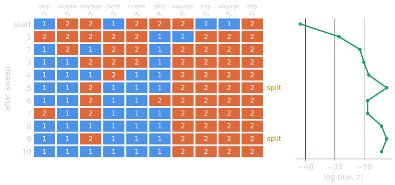
After ten sweeps the state has all of $d_1$ in the sea topic, which gives $\hat{\phi}_1 = (0.328, 0.168, 0.328, 0.168, 0.008)$ for ship, boat, ocean, voyage, trip and $\hat{\phi}_2 = (0.012, 0.012, 0.012, 0.482, 0.482)$, and $\hat{\theta}_{d_1} = (3.1/3.2,\ 0.1/3.2) = (0.969, 0.031)$.
Checking the sampler against the exact posterior
Ten words with two topics have only $2^{10} = 1{,}024$ possible assignments, so here, unlike Reuters, the posterior can be computed exactly by evaluating the collapsed joint for each and normalizing. The most probable assignments are:
| Assignment | Posterior probability (each labeling) |
|---|---|
| Sea/travel split: $d_1$'s voyage with travel, its ship and ocean with sea | 0.124 |
| boat and ocean alone in one topic, everything else in the other | 0.052 |
| All of $d_1$ with the sea words | 0.051 |
Each appears twice, once with the sea in topic 1 and once in topic 2, because swapping the labels of the topics changes nothing in the model. The split has total probability 0.247. The probability that all three words of $d_1$ share a topic is 0.412: with $\alpha = 0.1$, the prior strongly prefers documents about one thing, and $d_1$ is ambiguous.
Over 30 runs (seeds 1 to 30) of 10,000 sweeps each, discarding the first 100, the share of sweeps spent at the split had median 0.250 (interquartile range 0.244 to 0.255), matching the exact 0.247. The first visit to the split came after a median of 5 sweeps (IQR 4 to 15, longest 34). The sampled average of $\hat{\phi}$, after matching each sample's topics to sea and travel, had a median over the 30 runs within 0.003 of the exact posterior mean in every entry. Two lessons carry over to real collections. A single sample is one plausible state, not the answer: the posterior here is spread over many states. And averaging samples requires care, because topic labels can swap between samples. In this tiny example they swap often; in a large collection a swap within one run is rare, which is why topics are commonly reported from a single late sample, as Griffiths and Steyvers (2004) did.
Variational inference
Blei, Ng, and Jordan (2003) instead approximated the posterior with a simpler distribution in which the latent variables are independent, and adjusted that distribution to be as close as possible to the true posterior, by maximizing a lower bound on the likelihood of the data. The procedure resembles EM, alternating between updating each document's variational parameters and the topics.
For one document, the approximation gives $\theta$ its own Dirichlet with parameters $\gamma$, and each word position $n$ its own distribution $\varphi_n$ over topics (written $\phi$ in the paper, which uses $\beta$ for the topics). Minimizing the Kullback–Leibler divergence to the true posterior leads to two updates, repeated until they stop changing (Blei, Ng, and Jordan, 2003, §5.2, eqs. 6 to 8):
$$\varphi_{n,k} \propto \beta_{k, w_n} \exp\!\left( \Psi(\gamma_k) - \Psi\!\left(\textstyle\sum_j \gamma_j\right) \right), \qquad \gamma_k = \alpha_k + \sum_{n} \varphi_{n,k},$$
where $\beta_{k,w}$ is topic $k$'s probability for word $w$ and $\Psi$ is the digamma function, the derivative of $\log \Gamma$. They mirror the Gibbs update. The first is Bayes' rule for one word's topic, with the document's topic weight replaced by the exponential of its expected logarithm. The second is the conjugate update, the prior plus expected counts, with soft counts $\varphi$ in place of the sampler's hard assignments. The topics are then re-estimated from the expected counts of all documents, as in pLSA's M-step.
Online variational inference (Hoffman, Blei, and Bach, 2010) updates the topics from small batches of documents at a time, so it can process collections too large to hold in memory, or streams of new documents. The scikit-learn implementation used below offers both batch and online variants.
Hyperparameters
The values of $\alpha$ and $\beta$ affect the topics found, and they can be learned from the data instead of fixed. Wallach, Mimno, and McCallum (2009) found that an asymmetric prior on the document proportions, letting some topics be generally more common than others, gave better models and absorbed common words into a few general topics, while the prior on the topics could safely stay symmetric.
Twenty topics in Reuters
LDA was fitted to the 7,769 training stories of Reuters-21578, after lowercasing, keeping words of at least three letters, removing English stop words and a few Reuters-specific abbreviations (mln, dlrs, pct, shr, and others), and keeping the 6,855 words that appear in at least 5 stories and at most half of them. The model used $K = 20$, priors $\alpha = \beta = 1/K$, and 30 passes of batch variational inference. The labels below are interpretations of the top words. The average weight is the topic's mean proportion across stories, each story counting equally. The category is the one most common among the stories where the topic has the largest weight, with the share of those stories that carry it; stories can have several categories.
| Topic | Top words | Average weight | Most common category |
|---|---|---|---|
| Earnings tables | loss profit qtr revs oper note avg shrs sales includes | 15.6% | earn (98%) |
| Interest rates | bank rate banks market money rates central dealers fed week | 7.4% | interest (46%) |
| Asset sales | unit sale acquisition agreement sell assets terms subsidiary completed purchase | 7.0% | acq (89%) |
| Currencies and Japan | dollar japan economic government yen exchange japanese trade foreign currency | 6.4% | money-fx (40%) |
| Dividends | april record div gold pay qtly prior march sets dividend | 6.2% | earn (93%) |
| Economic statistics | january february rose rise stg december fell deficit compared surplus | 6.1% | trade (18%) |
| Grain and commodities | tonnes sugar wheat corn export usda production prices week grain | 5.3% | grain (51%) |
| Earnings reports | quarter earnings share sales profit expects reported results income profits | 5.1% | earn (94%) |
| Stakes | shares stock stake group common investment securities share exchange outstanding | 5.0% | acq (91%) |
| Takeover bids | offer share shares merger board tender shareholders bid stock acquisition | 4.9% | acq (93%) |
| Trade policy | trade japan states united house japanese usair officials reagan countries | 4.8% | trade (48%) |
| Metals and mixed | francs prices new plant steel marks copper price capacity group | 4.0% | crude (21%) |
| Stock splits | stock dividend split share april board record shareholders declared common | 3.6% | earn (91%) |
| Oil markets | oil opec bpd crude gulf prices saudi strike union ecuador | 3.2% | crude (56%) |
| British companies | stg plc group british standard shares bid pretax royal shell | 3.0% | earn (42%) |
| Soft commodities | coffee brazil cocoa prices stock producers new buffer export price | 2.9% | coffee (43%) |
| Energy production | oil gas energy reserves production petroleum exploration prices natural barrels | 2.8% | crude (58%) |
| Futures trading | analysts futures market analyst exchange american trading new contracts shearson | 2.6% | acq (35%) |
| (incoherent) | department dutch guilders credit hughes court baker bonus ccc turkey | 2.0% | acq (35%) |
| Agriculture abroad | china soviet grain wheat union crop weather state soybean agriculture | 2.0% | grain (56%) |
Most topics are immediately recognizable. Several patterns are typical of LDA:
- Large categories are split by their language. Earnings reports, the largest Reuters category, appear as four topics: results tables, dividend announcements, stock splits, and the prose of quarterly reports. Acquisitions appear as three: sales of units and assets, purchases of stakes, and takeover bids. As with K-means on Reuters, distinct vocabularies within one category are easier to separate than small categories with overlapping language.
- Topics follow co-occurrence, not meaning. "Trade policy" includes usair, which appears in 43 training stories, 42 of them about acquisitions, so its place in a trade topic is an artifact of the fit, not a theme. "Currencies and Japan" combines two subjects that often appeared in the same stories.
- Some topics are mixtures or junk. "Metals and mixed" combines steel, copper, and European currencies (francs and marks). One topic, of dutch, guilders, hughes, court, and turkey, has no coherent subject at all, and its coherence score, discussed in evaluating topic models, is the only negative one among the twenty.
What a topic is, in numbers
A list of ten words hides how a topic actually spreads its probability:
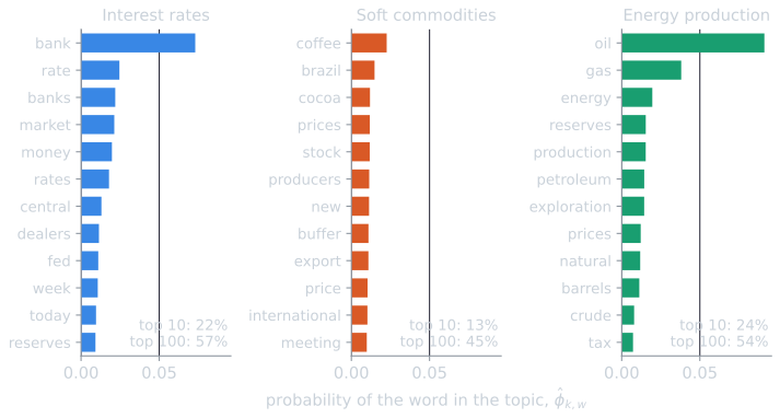
Across the twenty topics, the ten most probable words carry a median of 17 percent of a topic's probability, from 9 percent for "Currencies and Japan" to 55 percent for the formulaic "Earnings tables". In a typical topic about 870 words have more than the uniform probability $1/V$. The top-word lists are a summary for reading, and the tail is where most of the probability lives; that tail is what lets a topic give some probability to a word a document never used.
One story's mixture
The story training/1000, about a raised bid for Viacom, is labeled acq. Its inferred mixture is 35 percent takeover bids, 33 percent British companies, 19 percent stock splits, and 12 percent earnings tables. The first is right. The second is a mistake: nothing in the story concerns a British company. A short story gives inference little evidence, and words shared by several topics, such as bid, can be credited to the wrong one. Across the training set, 71 percent of stories had a single topic above one-half of their mixture, and stories had on average 2.3 topics with more than a tenth of their weight, which is close to what the prior with $\alpha = 1/K$ predicts, 2.25 topics above a tenth for random draws.
The scripts are reuters_lda.py, reuters_coherence_hand.py, and lda_gibbs_toy.py in tools/experiments/topics/ in the site repository, and the figures are drawn by tools/figures/latent-dirichlet-allocation.py.
References
- Blei, D. M., Ng, A. Y., and Jordan, M. I. (2003). Latent Dirichlet allocation. Journal of Machine Learning Research, 3, 993–1022.
- Griffiths, T. L., and Steyvers, M. (2004). Finding scientific topics. Proceedings of the National Academy of Sciences, 101(suppl. 1), 5228–5235.
- Hoffman, M. D., Blei, D. M., and Bach, F. (2010). Online learning for latent Dirichlet allocation. In Advances in Neural Information Processing Systems 23 (NIPS 2010), 856–864.
- McCallum, A. K. (2002). MALLET: A machine learning for language toolkit. Software, University of Massachusetts Amherst.
- Wallach, H. M., Mimno, D., and McCallum, A. (2009). Rethinking LDA: Why priors matter. In Advances in Neural Information Processing Systems 22 (NIPS 2009), 1973–1981.