Latent semantic indexing finds latent dimensions by minimizing squared error, a criterion with no natural interpretation for word counts. Its dimensions mix positive and negative values, and a document's coordinates are not proportions of anything. Hofmann (1999a, 1999b) kept LSI's idea, a small number of latent factors explaining word co-occurrence, and replaced the linear algebra with a probability model. Probabilistic latent semantic analysis (pLSA), called probabilistic latent semantic indexing (pLSI) when used for retrieval, was the first model to describe documents as mixtures of topics, each topic a distribution over words.
This article states the model, derives the expectation-maximization algorithm that fits it, and runs that algorithm by hand for two iterations on the five-term example of the LSI article.
The aspect model
pLSA introduces a hidden variable $z$, the topic or aspect, taking one of $K$ values. Each word occurrence in a document is explained by a topic: the document chooses a topic, and the topic chooses a word. The probability of word $w$ appearing in document $d$ is
$$P(w \mid d) = \sum_{z=1}^{K} P(w \mid z)\, P(z \mid d).$$
- $P(w \mid z)$ is the topic's distribution over words, shared by all documents.
- $P(z \mid d)$ is the document's mixture of topics, its own set of proportions.
The generative story
Hofmann (1999b, §3.1, eq. 1) defines the model as a joint distribution over document-word pairs, $P(d, w) = P(d) P(w \mid d)$ with $P(w \mid d)$ the mixture above. Read as a recipe, it generates the collection's word occurrences one $(d, w)$ pair at a time:
- Pick a document $d$ with probability $P(d)$.
- Pick a topic $z$ with probability $P(z \mid d)$.
- Pick a word $w$ with probability $P(w \mid z)$.
Only the pair $(d, w)$ is recorded; $z$ is discarded. The probability of a pair is $P(d, w) = P(d) \sum_z P(w \mid z) P(z \mid d)$. The model's one structural assumption is that $d$ and $w$ are conditionally independent given $z$: once the topic is known, which document the word came from tells nothing more about which word it is. Since $K$ is much smaller than the number of documents or words, $z$ acts as a bottleneck through which everything a document says about its words must pass.
By Bayes' rule, the same model can be written symmetrically in documents and words (Hofmann, 1999b, eq. 2):
$$P(d, w) = \sum_{z} P(z)\, P(d \mid z)\, P(w \mid z).$$
Here a topic is picked first, and it generates both a document and a word. The two forms define the same set of distributions. The symmetric one makes the resemblance to LSI plain, as Hofmann points out: written as matrices, it is $\hat{P} = U_z \Sigma_z V_z^{\mathsf{T}}$ with $U_z$ holding $P(d \mid z)$, $\Sigma_z$ the diagonal of $P(z)$, and $V_z$ holding $P(w \mid z)$, a factorization with the shape of the SVD but with every entry a probability.
The geometry
Each document's word distribution is a weighted average of $K$ topic distributions. With a vocabulary of $M$ words, every word distribution is a point in an $(M-1)$-dimensional simplex, and the model forces all of a collection's document distributions into the sub-simplex whose corners are the $K$ topics, of at most $K-1$ dimensions, which is the probabilistic counterpart of LSI's rank-$k$ subspace (Hofmann, 1999b, §3.3). Unlike LSI's dimensions, the topics and the mixture weights are probabilities: nonnegative, summing to 1, and readable as "this document is two-thirds about the sea".
With three words the simplex is a triangle and can be drawn. Restrict the example to ship, ocean, and voyage (dropping $d_6$, which contains none of them) and fit two topics:
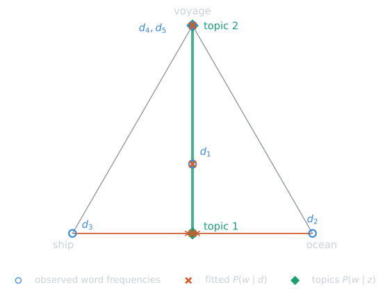
The best fit (log-likelihood −4.68, from 20 random starts) puts one topic at ship 0.5, ocean 0.5 and the other at voyage 1.0. Documents that the segment cannot reach are moved to the point on it that loses least likelihood; that loss is the price of describing five documents with two topics.
Fitting the model
With $n(d, w)$ the number of times word $w$ occurs in document $d$, the parameters are chosen to maximize the log-likelihood of the collection:
$$\mathcal{L} = \sum_{d} \sum_{w} n(d, w) \log \sum_{z} P(w \mid z)\, P(z \mid d).$$
(The factor $P(d)$ is dropped: its maximum-likelihood value is each document's share of the words, and it does not interact with the other parameters.) The sum inside the logarithm makes this hard to maximize directly. If the topic of every word occurrence were known, the estimates would be simple counts. They are not known, which is the situation expectation-maximization (EM) handles, as it did for the 2-Poisson model. Starting from random parameters, EM alternates two steps:
- E-step. For each document and word, compute the probability that each topic produced it: $$P(z \mid d, w) = \frac{P(w \mid z)\, P(z \mid d)}{\sum_{z'} P(w \mid z')\, P(z' \mid d)}.$$
- M-step. Re-estimate the parameters from the expected counts, as if each occurrence were divided among topics in those proportions: $$P(w \mid z) \propto \sum_{d} n(d, w)\, P(z \mid d, w), \qquad P(z \mid d) \propto \sum_{w} n(d, w)\, P(z \mid d, w).$$
Each round never decreases the likelihood, so EM converges, but, like K-means, only to a local maximum that depends on the starting point. Hofmann (1999b, eqs. 3 to 6) gives the same steps for the symmetric form, with $P(d \mid z)$ and $P(z)$ in place of $P(z \mid d)$.
Deriving the two steps
The updates are not guesses; they follow from a lower bound on $\mathcal{L}$.
- Introduce a distribution over topics for each pair. For every $(d, w)$, let $q_{dw}(z)$ be any probability distribution over the $K$ topics. Multiply and divide inside the logarithm: $$\log \sum_z P(w \mid z) P(z \mid d) = \log \sum_z q_{dw}(z)\, \frac{P(w \mid z) P(z \mid d)}{q_{dw}(z)}.$$
- Apply Jensen's inequality. The logarithm is concave, so the log of an average is at least the average of the logs: $$\log \sum_z q_{dw}(z)\, \frac{P(w \mid z) P(z \mid d)}{q_{dw}(z)} \;\ge\; \sum_z q_{dw}(z) \log \frac{P(w \mid z) P(z \mid d)}{q_{dw}(z)}.$$ Weighting by $n(d, w)$ and summing gives a lower bound $F(q, \text{parameters}) \le \mathcal{L}$ that holds for every choice of $q$.
- The E-step makes the bound tight. Jensen's inequality is an equality when the quantity being averaged is the same for every $z$, that is, when $q_{dw}(z)$ is proportional to $P(w \mid z) P(z \mid d)$. Normalizing gives exactly the posterior $P(z \mid d, w)$ of the E-step. With that $q$, $F = \mathcal{L}$ at the current parameters.
- The M-step maximizes the bound. With $q$ fixed, the parameters appear in $F$ only through $\sum_{d,w} n(d,w) \sum_z q_{dw}(z) \left[ \log P(w \mid z) + \log P(z \mid d) \right]$. Maximize the part containing $P(w \mid z)$ subject to $\sum_w P(w \mid z) = 1$ with a Lagrange multiplier $\lambda_z$: setting the derivative with respect to $P(w \mid z)$ to zero gives $\sum_d n(d,w) q_{dw}(z) / P(w \mid z) = \lambda_z$, so $P(w \mid z) = \sum_d n(d,w) q_{dw}(z) / \lambda_z$, and the constraint makes $\lambda_z$ the normalizing sum. The same argument for $P(z \mid d)$ gives the second update.
- Why the likelihood cannot fall. Write $\theta$ for the old parameters and $\theta'$ for the new. Then $\mathcal{L}(\theta') \ge F(q, \theta') \ge F(q, \theta) = \mathcal{L}(\theta)$: the first inequality is step 2, the second is step 4, and the equality is step 3.
Two consequences are visible in the derivation. EM climbs, but only to a point where no single E-step and M-step can improve; nothing guarantees that this is the global maximum. And a parameter that reaches zero stays at zero, since every update multiplies by it, so a start with zeros can never discover the words or topics it excluded.
Two iterations by hand
Run EM on the five-term example with $K = 2$ from a fixed start that leans slightly toward the sea in topic 1 and toward travel in topic 2, with every document's mixture even:
| ship | boat | ocean | voyage | trip | |
|---|---|---|---|---|---|
| $P(w \mid z_1)$ | 0.30 | 0.20 | 0.20 | 0.15 | 0.15 |
| $P(w \mid z_2)$ | 0.15 | 0.15 | 0.20 | 0.30 | 0.20 |
and $P(z_1 \mid d) = P(z_2 \mid d) = 0.5$ for all six documents. Every document then has the same predicted distribution, $P(w \mid d) = (0.225, 0.175, 0.200, 0.225, 0.175)$, and the log-likelihood of the ten word occurrences is $\mathcal{L} = -15.906$. Values below are from plsa_trace.py in tools/experiments/topics/, rounded to three or four decimals.
Iteration 1, E-step. For ship in $d_1$ the numerators are $P(\text{ship} \mid z_1) P(z_1 \mid d_1) = 0.30 \times 0.5 = 0.150$ and $0.15 \times 0.5 = 0.075$, so $P(z_1 \mid d_1, \text{ship}) = 0.150 / 0.225 = 0.667$. Because every mixture is still even, the posterior depends only on the word, and it is the same in every document:
| Word | ship | boat | ocean | voyage | trip |
|---|---|---|---|---|---|
| $P(z_1 \mid d, w)$ | 0.667 | 0.571 | 0.500 | 0.333 | 0.429 |
Iteration 1, M-step. Each occurrence is split between the topics in those proportions. ship occurs twice, so it contributes $2 \times 0.667 = 1.333$ expected occurrences to topic 1 and 0.667 to topic 2; voyage, three times, contributes 1.0 and 2.0. Topic 1 receives 4.762 expected occurrences in all and topic 2 receives 5.238. Dividing each word's expected count by its topic's total:
| ship | boat | ocean | voyage | trip | |
|---|---|---|---|---|---|
| $P(w \mid z_1)$ | 0.280 | 0.120 | 0.210 | 0.210 | 0.180 |
| $P(w \mid z_2)$ | 0.127 | 0.082 | 0.191 | 0.382 | 0.218 |
Each document's mixture is its share of expected occurrences. $d_3$ (ship) has one occurrence, 0.667 of it in topic 1, so $P(z_1 \mid d_3) = 0.667$. $d_1$ has 1.5 of its 3 occurrences in topic 1, so it stays at 0.5:
| $d_1$ | $d_2$ | $d_3$ | $d_4$ | $d_5$ | $d_6$ | |
|---|---|---|---|---|---|---|
| $P(z_1 \mid d)$ | 0.500 | 0.536 | 0.667 | 0.381 | 0.333 | 0.429 |
The log-likelihood rises to $-15.242$. The bound of the derivation shows the mechanism: at the old parameters, with $q$ the posterior, $F = -15.906 = \mathcal{L}$; at the new parameters with the same $q$, $F = -15.397$; and the true log-likelihood at the new parameters, $-15.242$, is higher still.
Iteration 2. Now the mixtures differ, so the same word gets different posteriors in different documents. For ship in $d_3$ the numerators are $0.280 \times 0.667 = 0.187$ and $0.127 \times 0.333 = 0.042$, so the posterior is 0.815; for ship in $d_1$, whose mixture is still even, it is 0.688. A document's other words pull each of its words toward the document's dominant topic:
| Occurrence | $P(z_1 \mid d, w)$ | Occurrence | $P(z_1 \mid d, w)$ |
|---|---|---|---|
| $d_1$ ship | 0.688 | $d_3$ ship | 0.815 |
| $d_1$ ocean | 0.524 | $d_4$ voyage | 0.253 |
| $d_1$ voyage | 0.355 | $d_4$ trip | 0.337 |
| $d_2$ boat | 0.629 | $d_5$ voyage | 0.216 |
| $d_2$ ocean | 0.559 | $d_6$ trip | 0.382 |
The M-step gives $P(w \mid z_1) = (0.316, 0.132, 0.228, 0.173, 0.151)$ and $P(w \mid z_2) = (0.095, 0.071, 0.175, 0.415, 0.244)$, and mixtures $P(z_1 \mid d) = (0.522, 0.594, 0.815, 0.295, 0.216, 0.382)$. The log-likelihood is $-14.678$.
Afterward. The separation feeds on itself. The log-likelihood over the first ten iterations is $-15.906$, $-15.242$, $-14.678$, $-13.571$, $-12.050$, $-10.970$, $-10.650$, $-10.589$, $-10.571$, $-10.563$, $-10.558$, and it settles at $-10.549$ by iteration 50. The final topics put ship 0.4, ocean 0.4, boat 0.2 in topic 1 and voyage 0.6, trip 0.4 in topic 2, with every other probability zero: the best solution described next.
The example
Applied to the five-term, six-document matrix of the LSI article (terms ship, boat, ocean, voyage, trip) with $K = 2$, EM run from 20 random starts reached four different solutions. The best one, with log-likelihood −10.55, found:
| Topic | Word probabilities |
|---|---|
| Sea | ship 0.40, ocean 0.40, boat 0.20 |
| Travel | voyage 0.60, trip 0.40 |
Documents $d_2$ (boat ocean) and $d_3$ (ship) are entirely sea, and $d_4$, $d_5$, and $d_6$ entirely travel. Document $d_1$, containing ship, ocean, and voyage, is two-thirds sea and one-third travel. The topics are the same division LSI's second dimension found, but expressed as distributions with no negative values. Each probability is a simple count: the sea topic received the five sea-word occurrences (two of ship, one of boat, two of ocean), and the travel topic the three of voyage and two of trip. The other starts converged to worse solutions, with log-likelihoods −11.37, −11.61, and −12.14, showing the local maxima directly. The script is plsa_toy.py in tools/experiments/topics/.
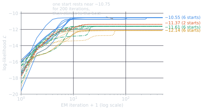
Six of the 20 starts found the best solution, two reached −11.37, six −11.61, and six −12.14. The usual remedy is the one used here: run EM from many starts and keep the best.
Using it for retrieval
For retrieval, Hofmann (1999a) compared queries and documents through their topic mixtures, and combined the result with ordinary term matching. He reported better retrieval than LSI on four small test collections, among them Cranfield. A query, being a new document, has no $P(z \mid d)$ of its own. It is folded in by running EM on the query alone with the topics $P(w \mid z)$ held fixed. For the query boat ocean and the best solution above, both words have probability zero in the travel topic, so folding in gives the query a mixture of entirely sea, the same as $d_2$ and $d_3$, and both would be retrieved, as LSI retrieved them.
Relation to other methods
pLSA sits between LSI and the models that followed:
- LSI. Both factor the term-document matrix into $K$ factors. LSI minimizes squared error, which corresponds to Gaussian noise, and allows negative values. pLSA maximizes a multinomial likelihood, suited to counts, and keeps everything nonnegative.
- Nonnegative matrix factorization. Factoring a nonnegative matrix into two nonnegative matrices, with the generalized Kullback–Leibler divergence as the measure of error, optimizes the same objective as pLSA, and a pLSA solution is, after normalization, a solution of that NMF problem (Gaussier and Goutte, 2005). NMF is described in topic models beyond LDA.
- LDA. pLSA is a special case of LDA, the maximum a posteriori estimate when the Dirichlet prior on topic mixtures is uniform (Girolami and Kabán, 2003).
Why pLSA was not the end
Two weaknesses, identified by Blei, Ng, and Jordan (2003), led to latent Dirichlet allocation:
- The number of parameters grows with the collection. Every document has its own $K - 1$ free mixture weights, in addition to the $K(M - 1)$ topic parameters, so a collection of $N$ documents has $K(M-1) + N(K-1)$ parameters. In the example that is $2 \times 4 + 6 \times 1 = 14$ parameters for 10 word occurrences. A model with so much freedom fits the training documents closely and overfits: the best solution above gives five of the six documents a mixture of exactly 0 or 1, and so says that $d_2$ and $d_3$ could never contain the word trip, or $d_4$ the word ship: $P(\text{trip} \mid d_2) = 0$. Hofmann used tempered EM, which raises the E-step's joint probabilities to a power $\beta < 1$ before normalizing, softening the posteriors and so the fit (Hofmann, 1999b, §3.6), to reduce the problem.
- It is not a model of documents. The mixtures $P(z \mid d)$ are parameters attached to the training documents, with no account of where they come from. There is no principled probability for a new document, only the folding-in procedure, which fits new parameters for it.
LDA addresses both by treating each document's mixture as a random draw from a shared Dirichlet distribution. The number of parameters then depends only on $K$ and the vocabulary, and any document, seen or unseen, has a probability under the model.
The figures are drawn by tools/figures/probabilistic-latent-semantic-analysis.py.
References
- Blei, D. M., Ng, A. Y., and Jordan, M. I. (2003). Latent Dirichlet allocation. Journal of Machine Learning Research, 3, 993–1022.
- Gaussier, E., and Goutte, C. (2005). Relation between PLSA and NMF and implications. In Proceedings of SIGIR 2005, 601–602.
- Girolami, M., and Kabán, A. (2003). On an equivalence between PLSI and LDA. In Proceedings of SIGIR 2003, 433–434.
- Hofmann, T. (1999a). Probabilistic latent semantic indexing. In Proceedings of SIGIR 1999, 50–57.
- Hofmann, T. (1999b). Probabilistic latent semantic analysis. In Proceedings of the Fifteenth Conference on Uncertainty in Artificial Intelligence (UAI 1999), 289–296.