The training stories of the Reuters-21578 collection contain 18,135 distinct terms after stemming. A classifier deciding whether a story is about grain does not need most of them. Wheat, tonne, corn, and USDA say a great deal about grain, while Tuesday and spokesman say nothing. Feature selection keeps a subset of the terms and discards the rest before the classifier is trained. This article explains the reasons for doing so, works the two standard measures for choosing terms by hand on real counts, and shows what selection actually does to accuracy on Reuters, which turns out to be less than the textbook suggests, for a reason that a small experiment pins down.
Why select features
Feature selection serves two purposes (Manning, Raghavan, and Schütze, 2008, §13.5):
- Efficiency. Fewer features mean smaller models and faster training and classification. For methods whose cost grows with the number of features, the saving can be large.
- Removing noise features. A term that by chance occurs more often in one class's training documents can mislead the classifier on new documents, a form of overfitting. Removing such noise features can improve accuracy.
The usual procedure is simple. For each class, compute a utility score for every term, rank the terms by it, and keep the top $k$. In a multilabel setting, each binary classifier gets its own set of features. The measures differ in what "utility" means. All the measures in this article start from the same four numbers for each term and class, so it is worth setting them out first.
The two-by-two table
For a term $t$ and a class $c$, every training document falls into one of four cells, according to whether it contains the term and whether it belongs to the class:
| In class $c$ | Not in class $c$ | Total | |
|---|---|---|---|
| Contains $t$ | $N_{11}$ | $N_{10}$ | $N_{1.}$ |
| Lacks $t$ | $N_{01}$ | $N_{00}$ | $N_{0.}$ |
| Total | $N_{.1}$ | $N_{.0}$ | $N$ |
The first subscript records the term and the second the class. $N_{1.} = N_{11} + N_{10}$ is the number of documents containing the term, $N_{.1} = N_{11} + N_{01}$ the number in the class, and similarly for $N_{0.}$ and $N_{.0}$. For the term wheat and the Reuters category grain, counted over the 7,769 training stories:
| In grain | Not in grain | Total | |
|---|---|---|---|
| Contains wheat | 227 | 16 | 243 |
| Lacks wheat | 206 | 7,320 | 7,526 |
| Total | 433 | 7,336 | 7,769 |
Wheat appears in 243 stories, 227 of them about grain. A term that told nothing about the class would be spread across the columns in proportion to the column totals: since 433/7,769 = 5.6 percent of stories are about grain, about 5.6 percent of the stories containing it would be, or 13.5 of 243. The measures below quantify how far the observed table departs from that.
Mutual information
Mutual information (MI) measures how much knowing whether a term occurs in a document reduces uncertainty about whether the document belongs to the class. Let $U$ be a random variable that is 1 if the document contains term $t$ and 0 otherwise, and $C$ one that is 1 if the document is in class $c$ and 0 otherwise. Then
$$I(U; C) = \sum_{e_t \in \{1, 0\}} \sum_{e_c \in \{1, 0\}} P(U = e_t, C = e_c) \log_2 \frac{P(U = e_t, C = e_c)}{P(U = e_t)\, P(C = e_c)}.$$
The ratio inside the logarithm compares how often a cell occurs with how often it would occur if term and class were independent. The measure is zero when the term's occurrence is independent of the class and largest when the term predicts the class perfectly. Estimating each probability by its count divided by $N$ gives
$$I = \frac{N_{11}}{N} \log_2 \frac{N N_{11}}{N_{1.} N_{.1}} + \frac{N_{01}}{N} \log_2 \frac{N N_{01}}{N_{0.} N_{.1}} + \frac{N_{10}}{N} \log_2 \frac{N N_{10}}{N_{1.} N_{.0}} + \frac{N_{00}}{N} \log_2 \frac{N N_{00}}{N_{0.} N_{.0}}.$$
A cell with a count of zero contributes zero, since $x \log x \to 0$ as $x \to 0$. The other three cells must still be included. Skipping the whole term when one cell is zero is a common implementation mistake.
Worked by hand: wheat and grain
Each cell of the wheat table contributes one term of the sum (computed by tools/experiments/reuters/fs_worked.py; ratios to four decimals, contributions to five):
| Cell | $N_{e_t e_c}/N$ | Ratio $N N_{e_t e_c} / (N_{e_t .} N_{. e_c})$ | $\log_2$ of ratio | Contribution |
|---|---|---|---|---|
| contains, in grain | 227/7,769 = 0.0292 | 7,769 × 227 / (243 × 433) = 16.7609 | +4.0670 | +0.11883 |
| contains, not in grain | 16/7,769 = 0.0021 | 0.0697 | −3.8421 | −0.00791 |
| lacks, in grain | 206/7,769 = 0.0265 | 0.4911 | −1.0259 | −0.02720 |
| lacks, not in grain | 7,320/7,769 = 0.9422 | 1.0300 | +0.0427 | +0.04023 |
| Total | 0.12395 bits |
The first cell dominates: stories containing wheat are 16.8 times more likely to be about grain than independence predicts. Two contributions are negative, because those cells occur less often than independence predicts, but the total is never negative. With 0.124 bits, wheat ranks first among all 18,135 terms for grain.
The textbook's example
Manning, Raghavan, and Schütze (2008, §13.5.1) take the class poultry and the term export in the Reuters-RCV1 collection:
| In poultry | Not in poultry | |
|---|---|---|
| Contains export | $N_{11} = 49$ | $N_{10} = 27{,}652$ |
| Lacks export | $N_{01} = 141$ | $N_{00} = 774{,}106$ |
With $N = 801{,}948$, the formula gives $I \approx 0.0001105$ bits. The value is tiny in absolute terms because poultry is a rare class, so even a perfect predictor of it could remove little uncertainty about a random document. Only the ranking of MI values among terms matters for selection.
Negative association counts too
Mutual information rewards any departure from independence, in either direction. The fourth-ranked term for grain shows what that means:
| In grain | Not in grain | Total | |
|---|---|---|---|
Contains lt |
2 | 4,316 | 4,318 |
Lacks lt |
431 | 3,020 | 3,451 |
lt is not a word. It is a fragment of the HTML entity <, which the Reuters text uses to encode the opening angle bracket before company names, so it appears in more than half the training stories. Only 2 of them are about grain. Its MI of 0.06573 bits comes from the two cells that record negative association: grain stories lack it 2.24 times as often as independence predicts, which contributes +0.06458, and other stories contain it slightly more often than predicted, +0.04559. The other two cells subtract 0.04443. The presence of lt is evidence against grain. Its absence is mild evidence for it, since almost every grain story lacks it. For selection this distinction matters, as the experiment below shows.
Mutual information in this sense, an expectation over all four cells, is what other authors call information gain. The name "mutual information" is sometimes used instead for the pointwise quantity $\log \frac{P(t, c)}{P(t)\,P(c)}$, which looks at only one cell. In Yang and Pedersen's (1997) comparison, information gain was among the best selection measures and pointwise mutual information among the worst, because it favors rare terms. Comparisons across papers should check which quantity is meant.
The χ² statistic
The χ² test of independence asks whether the term's occurrence and the class's occurrence are independent. It compares the observed count in each cell with the count expected if they were:
$$X^2 = \sum_{e_t \in \{0, 1\}} \sum_{e_c \in \{0, 1\}} \frac{(N_{e_t e_c} - E_{e_t e_c})^2}{E_{e_t e_c}},$$
where the expected count $E_{e_t e_c}$ is $N$ times the product of the two marginal probabilities, which simplifies to the row total times the column total divided by $N$. For wheat and grain:
| Cell | Observed | Expected | $(O - E)^2 / E$ |
|---|---|---|---|
| contains, in grain | 227 | 243 × 433 / 7,769 = 13.54 | 3,364.3 |
| contains, not in grain | 16 | 243 × 7,336 / 7,769 = 229.46 | 198.6 |
| lacks, in grain | 206 | 7,526 × 433 / 7,769 = 419.46 | 108.6 |
| lacks, not in grain | 7,320 | 7,526 × 7,336 / 7,769 = 7,106.54 | 6.4 |
| Total | $X^2 = 3{,}677.9$ |
As with mutual information, the cell for documents that contain the term and are in the class carries most of the weight. For a two-by-two table the four cells collapse to a direct formula:
$$X^2 = \frac{N (N_{11} N_{00} - N_{10} N_{01})^2}{(N_{11} + N_{01})(N_{11} + N_{10})(N_{10} + N_{00})(N_{01} + N_{00})},$$
which gives the same 3,677.9. The numerator's $N_{11} N_{00} - N_{10} N_{01}$ is zero exactly when the table matches independence, and it is squared, so χ², like mutual information, rewards association in either direction.
For the textbook's export and poultry, the expected count of documents in both is
$$E_{11} = N \times \frac{N_{1.}}{N} \times \frac{N_{.1}}{N} \approx 6.6,$$
but 49 are observed. The formula gives $X^2 \approx 284$, far above 10.83, the value needed to reject independence at the 0.001 level. Export is strongly associated with poultry, as one might expect for a category about the poultry trade.
χ² is a statistical test used here as a ranking score. The statistical objections to that use, such as the many tests run at once and the missing continuity correction for a two-by-two table, matter little, since only the ranking is used, not the significance level (Manning, Raghavan, and Schütze, 2008, §13.5.2). A real weakness is that a test of significance favors rare terms. A term that occurs in only a few documents, all of them in the class, is highly significant but says little about most documents, so χ² selects more such rare terms than mutual information does (§13.5.5).
Frequency
The simplest measure keeps the terms that occur in the most documents of the class, the $N_{11}$ cell alone. It is cheap, and it removes rare terms that are likely to be noise. But it also keeps common words that occur everywhere, which have no power to distinguish the class. From occurs in 210 of the 433 grain stories, but also in 2,782 others, close to the 166.8 grain stories expected by chance; its MI is 0.00175 bits and its χ² 19.3, ranking 340th and 605th.
What each method selects
For the Reuters category grain, the ten terms each method chose from the training stories, after stemming:
| Method | Top ten terms |
|---|---|
| Mutual information | agricultur, corn, crop, depart, export, grain, lt, tonn, usda, wheat |
| χ² | agricultur, barlei, corn, crop, farmer, grain, maiz, tonn, usda, wheat |
| Frequency | agricultur, corn, export, from, grain, ha, mln, tonn, wheat, year |
χ² picks the most specific vocabulary, such as barley, maize, and farmer. Frequency picks generic words that happen to be common in grain stories, such as from, has (stemmed to ha), mln, and year. Mutual information's list includes lt, for the reason shown above: its absence is informative, and mutual information ranks it fourth. χ² gives it 564.3 and ranks it 13th, just outside its top ten. The example is a reminder that feature selection inherits every artifact of tokenization.
The textbook's remark that χ² prefers rarer terms can be seen by plotting every term's score against the number of training stories that contain it:
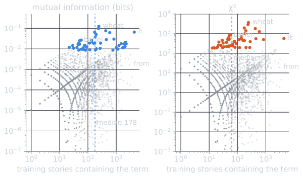
Under χ², the 50 selected terms have a median document frequency of 63; under mutual information, 178. The two lists share 37 of their 50 terms. The preference is relative, not extreme: none of χ²'s top 100 terms for grain occurs in fewer than four training stories.
The effect on accuracy
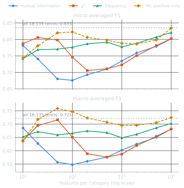
Multinomial Naive Bayes was trained on the ten largest Reuters categories with the top $k$ features per category under each measure, and evaluated on the standard test stories:
| Features per category | MI micro / macro F1 | χ² micro / macro F1 | Frequency micro / macro F1 |
|---|---|---|---|
| 10 | 0.781 / 0.686 | 0.787 / 0.638 | 0.742 / 0.652 |
| 50 | 0.680 / 0.557 | 0.798 / 0.716 | 0.771 / 0.659 |
| 100 | 0.676 / 0.548 | 0.746 / 0.651 | 0.776 / 0.666 |
| 500 | 0.710 / 0.576 | 0.711 / 0.576 | 0.792 / 0.668 |
| 1,000 | 0.735 / 0.602 | 0.723 / 0.587 | 0.778 / 0.649 |
| 5,000 | 0.779 / 0.650 | 0.781 / 0.654 | 0.807 / 0.686 |
| All 18,135 | 0.835 / 0.721 |
With these three measures, no feature set beat using all the features. The textbook reports that on a larger Reuters collection, RCV1, multinomial Naive Bayes with 10 to 100 features selected by mutual information outperformed the same classifier with all features by about 0.1 in F1 (Manning, Raghavan, and Schütze, 2008, §13.5.1). That did not happen here, and the curves are not even monotonic. Mutual information does worst between 50 and 100 features, where χ² does best.
Why mutual information fails here: an experiment
A plausible reason is the one lt illustrates. Mutual information rewards negative association as well as positive, so it selects terms whose absence indicates the class. A multinomial classifier can only use the terms present in a document: a term the document lacks adds nothing to its score, as Naive Bayes classification shows. A negatively associated term in the feature set therefore contributes only when it is present, which is when it counts against the class, and it never contributes the positive evidence that made it rank highly. Such features waste much of a small budget. Among the top 50 terms by mutual information, 29 are negatively associated for earn, 15 for acq, and between 6 and 12 for each of the other eight categories.
The explanation predicts that restricting mutual information to positively associated terms, those with $N_{11} N_{00} > N_{10} N_{01}$, should remove the dip. It does:
| Features per category | MI, positive terms only, micro / macro F1 | MI, all terms, micro / macro F1 |
|---|---|---|
| 10 | 0.744 / 0.635 | 0.781 / 0.686 |
| 50 | 0.820 / 0.759 | 0.680 / 0.557 |
| 100 | 0.822 / 0.747 | 0.676 / 0.548 |
| 500 | 0.798 / 0.707 | 0.710 / 0.576 |
| 1,000 | 0.788 / 0.695 | 0.735 / 0.602 |
| 5,000 | 0.799 / 0.705 | 0.779 / 0.650 |
| 10,000 | 0.834 / 0.724 | 0.802 / 0.681 |
At 50 features per category, the restricted measure scores 0.820 micro-F1 and 0.759 macro-F1, against 0.680 and 0.557 for unrestricted mutual information. Its macro-F1 is above the full vocabulary's 0.721, so selection does improve the small categories here, as in the textbook's experiment, once the measure suits the classifier. Micro-F1 stays slightly below the full vocabulary's 0.835. These numbers were read off the test set at a handful of values of $k$, so the best of them is an optimistic estimate; the point is the shape of the curves: the restricted measure beats unrestricted mutual information at every size from 20 to 10,000 features. The Bernoulli model, which uses absent terms as well as present ones, has no such problem with mutual information, and its accuracy is highest with 10 to 20 features.
What selection buys
The results still show the main practical value of selection. With only 50 features per category, 0.3 percent of the vocabulary, χ² selection came within 0.005 of the full model's macro-F1, though 0.037 below it on micro-F1, and the result was sensitive to the exact number of features. Yang and Pedersen (1997) reported the same finding with other classifiers: information gain and χ² could remove the great majority of terms with little or no loss of accuracy. Selection buys efficiency cheaply, and whether it also improves accuracy depends on the classifier, the collection, and the measure. Forman (2003), in a larger comparison, found a measure called bi-normal separation best overall, especially for highly skewed classes, with information gain a strong choice when only a few features are kept. The Bernoulli model, whose scores multiply over every vocabulary term, benefits from selection far more than the multinomial model does.
Selecting on training data only
Feature selection uses the class labels, so it is part of training. Selecting features using all the labeled data, then splitting the data for training and testing or for cross-validation, lets the test labels influence which features the classifier sees. Test results then overstate how the classifier will do on new data. Selection must be repeated inside each training split, using only that split's labels (see evaluating classifiers). All the tables in this article were computed this way: the counts come from the 7,769 training stories only.
References
- Forman, G. (2003). An extensive empirical study of feature selection metrics for text classification. Journal of Machine Learning Research, 3, 1289–1305.
- Manning, C. D., Raghavan, P., and Schütze, H. (2008). Introduction to Information Retrieval, section 13.5. Cambridge University Press.
- Yang, Y., and Pedersen, J. O. (1997). A comparative study on feature selection in text categorization. In Proceedings of ICML 1997, 412–420.