Two optimizers are run on the same problem with two objectives, both to be minimized, whose true Pareto front is the line $f_1 + f_2 = 1$ for $0 \le f_1 \le 1$. The first returns six points that lie exactly on the front, but all of them between $f_1 = 0.4$ and $f_1 = 0.6$. The second returns six points spread evenly from one end of the front to the other, but each sits $0.1$ behind it in both objectives. Which result is better? Neither set dominates the other: each contains points that no point of the other set beats. Under Pareto dominance the two are simply incomparable, and yet papers comparing multi-objective evolutionary algorithms must rank them.
A quality indicator settles the question by mapping a set of objective vectors to a single number. A good approximation of a front is usually expected to be close to it, to cover its whole extent, and to spread its points over it rather than bunching them, although no list of such criteria defines quality exactly (Zitzler, Thiele, Laumanns, Fonseca, and Grunert da Fonseca, 2003). Different indicators weigh these properties differently, and on the example above they split almost evenly. This article defines the most common indicators, computes them on four constructed fronts, shows where and why they disagree, and summarizes what can be proved about indicators of this kind.
Setting and notation
All objectives are minimized. An optimizer's output is an approximation set $A = \{\mathbf{a}_1, \dots, \mathbf{a}_n\}$ of mutually non-dominated objective vectors in $m$ dimensions. Several indicators also need a reference set $Z = \{\mathbf{z}_1, \dots, \mathbf{z}_k\}$, a dense, evenly spaced sample of the true front, which is known for benchmark problems and unknown for most real ones. The hypervolume needs instead a single reference point $\mathbf{r}$, worse than every point of interest in every objective.
The examples use four fronts on the line $f_1 + f_2 = 1$, each with six points:
- A, even: $f_1 = 0, 0.2, 0.4, 0.6, 0.8, 1$, on the front.
- B, clustered: $f_1 = 0.40, 0.44, \dots, 0.60$, on the front but covering a fifth of it.
- C, shifted: the points of A moved by $+0.1$ in both objectives, so every point of C is dominated by a point of A.
- D, uneven: $f_1 = 0, 0.05, 0.1, 0.15, 0.2, 1$, on the front, with both ends covered but a large gap.
The reference set $Z$ is 101 evenly spaced points on the front, and the hypervolume reference point is $(1.1, 1.1)$.
Hypervolume
The hypervolume of $A$ is the size of the region of objective space that $A$ dominates, bounded by the reference point:
$$\mathrm{HV}(A) = \lambda\Big( \bigcup_{\mathbf{a} \in A} [a_1, r_1] \times [a_2, r_2] \times \dots \times [a_m, r_m] \Big),$$
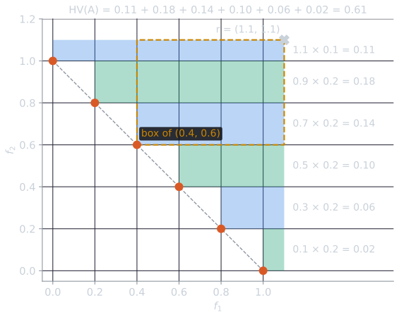
where $\lambda$ is Lebesgue measure: area for two objectives, volume for three. Larger is better. Zitzler and Thiele (1998) introduced it as the "size of the space covered" and used it again to compare algorithms when they proposed the strength Pareto evolutionary algorithm (Zitzler and Thiele, 1999). Each point contributes a box reaching to the reference point, and the hypervolume is the area of the union of the boxes. In two dimensions the union is a staircase. For the even front A, sorting the points by $f_1$ and adding horizontal strips gives
$$\mathrm{HV}(A) = 1.1 \times 0.1 + (0.9 + 0.7 + 0.5 + 0.3 + 0.1) \times 0.2 = 0.610.$$
The sweep behind that sum is simple enough to do by hand. Sort the points by $f_1$. Keep a running value, the lowest $f_2$ seen so far, starting at the reference point's $r_2$. Each point then adds a horizontal strip: its width runs from the point to the reference point, $r_1 - f_1$, and its height is the drop from the running value to the point's own $f_2$. A point whose $f_2$ is not below the running value is dominated and adds nothing. For A, the script tools/experiments/evolution/indicators_worked.py gives:
| Point | Width $r_1 - f_1$ | Height | Strip area | Exclusive contribution |
|---|---|---|---|---|
| (0.0, 1.0) | 1.1 | 0.1 | 0.110 | 0.020 |
| (0.2, 0.8) | 0.9 | 0.2 | 0.180 | 0.040 |
| (0.4, 0.6) | 0.7 | 0.2 | 0.140 | 0.040 |
| (0.6, 0.4) | 0.5 | 0.2 | 0.100 | 0.040 |
| (0.8, 0.2) | 0.3 | 0.2 | 0.060 | 0.040 |
| (1.0, 0.0) | 0.1 | 0.2 | 0.020 | 0.020 |
| Total | 0.610 | 0.200 |
The strips are not the points' own contributions. The first strip, for example, also contains area that $(0.2, 0.8)$ dominates. The last column answers a different question: how much hypervolume would be lost if that one point were removed. In two dimensions this exclusive contribution is the rectangle between a point and its two neighbours, $(f_1^{\text{next}} - f_1) \times (f_2^{\text{prev}} - f_2)$, with the reference point standing in for a missing neighbour at either end. An interior point of A owns a $0.2 \times 0.2$ square; an end point owns only $0.2 \times 0.1$, because the reference point is 0.1 beyond it. The exclusive contributions add up to 0.200, much less than the total, since most of the region is dominated by several points at once. Algorithms that select on the hypervolume, such as SMS-EMOA in multi-objective evolutionary algorithms, discard, from the worst-ranked front, the point with the smallest exclusive contribution.
The hypervolume is popular because it respects dominance. Zitzler et al. (2003) call one approximation set better than another if every point of the second is weakly dominated by some point of the first and the reverse does not hold. They showed that if $A$ is better than $B$, then $\mathrm{HV}(A) > \mathrm{HV}(B)$: $A$ must contain a point that $B$ does not weakly dominate, and some region is dominated by that point and by nothing in $B$. An indicator with this property is called Pareto compliant, and the hypervolume is the only widely used unary indicator known to have it (Ishibuchi, Masuda, Tanigaki, and Nojima, 2015). The guarantee runs in one direction only. $\mathrm{HV}(A) > \mathrm{HV}(B)$ shows that $B$ is not better than $A$, but the two may still be incomparable, as B and C are. The guarantee also assumes that the points lie inside the box bounded by $\mathbf{r}$. A point that does not strictly dominate the reference point contributes nothing, however good it is in the other objectives.
The reference point changes the ranking
That last caveat has practical consequences. Take two sets of four points, both on the true front:
- P includes both ends: $f_1 = 0, \tfrac{1}{3}, \tfrac{2}{3}, 1$.
- Q keeps away from the ends: $f_1 = 0.125, 0.375, 0.625, 0.875$.
No point of either set dominates a point of the other. With the reference point at $(r, r)$, summing the strips gives $\mathrm{HV}(P) = r^2 - \tfrac{2}{3}$ and $\mathrm{HV}(Q) = r^2 - \tfrac{r}{4} - \tfrac{23}{64}$, so
$$\mathrm{HV}(P) - \mathrm{HV}(Q) = \frac{r}{4} - \frac{59}{192},$$
which changes sign at $r = 59/48 \approx 1.229$.
| Reference point | HV(P) | HV(Q) | Larger |
|---|---|---|---|
| (1.0, 1.0) | 0.3333 | 0.3906 | Q |
| (1.1, 1.1) | 0.5433 | 0.5756 | Q |
| (1.2, 1.2) | 0.7733 | 0.7806 | Q |
| (1.3, 1.3) | 1.0233 | 1.0056 | P |
| (1.5, 1.5) | 1.5833 | 1.5156 | P |
| (2.0, 2.0) | 3.3333 | 3.1406 | P |
At the nadir point $(1, 1)$, the end points of P lie on the boundary of the box and add nothing, so Q, with all four points in the interior, wins. As the reference point moves away, the boxes of the end points grow with it, and P overtakes Q.
The strip sums show the mechanism. At $r = 1.0$, only P's two interior points count: $\tfrac{2}{3} \times \tfrac{1}{3} + \tfrac{1}{3} \times \tfrac{1}{3} = 0.3333$. At $r = 1.3$, all four count: $1.3 \times 0.3 + 0.9667 \times \tfrac{1}{3} + 0.6333 \times \tfrac{1}{3} + 0.3 \times \tfrac{1}{3} = 1.0233$. Each end point of P now owns a $0.3 \times \tfrac{1}{3}$ rectangle, 0.1 of area, that no other point covers. In general, moving the reference point out adds a band along the top of the box and a band along its right side. The top band starts at the set's smallest $f_1$, and the right band at its smallest $f_2$. P reaches $f_1 = 0$ and $f_2 = 0$, so its bands run the full width of the box; Q's start 0.125 in from each axis. From $r = 1.0$ to $r = 1.3$, P gains $1.0233 - 0.3333 = 0.69$ and Q gains $1.0056 - 0.3906 = 0.615$, and the difference is the two missing pieces, $2 \times 0.125 \times 0.3 = 0.075$. That is why the gap between the two hypervolumes grows linearly in $r$, with slope $2 \times 0.125 = \tfrac{1}{4}$, as the formula above says.
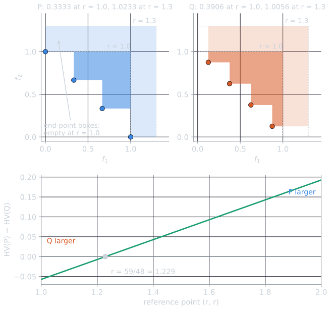
Neither choice is wrong; they encode different preferences about the ends of the front. A reference point "slightly worse than the nadir point" is the usual convention, and Ishibuchi, Imada, Setoguchi, and Nojima (2018) show that it is not always appropriate for fair comparison and propose a principled way to choose it. A comparison that reports hypervolumes without the reference point, and without the normalization applied to the objectives, cannot be reproduced. Since the hypervolume multiplies quantities measured in each objective's units, an objective with a large range dominates the volume, and a reference point set a fixed distance beyond the nadir sits at a different relative position in each objective, so objectives are usually normalized first.
Computational cost
In two dimensions the staircase needs only a sort, so the hypervolume costs $O(n \log n)$. In general it is hard. Computing the volume of a union of axis-parallel boxes that share a common corner, which is exactly the hypervolume, is #P-hard (Bringmann and Friedrich, 2010), so no exact algorithm can run in time polynomial in both the number of points and the number of objectives unless P = NP. Exact algorithms therefore trade on structure. The WFG algorithm adds the points one at a time and computes the volume each new point contributes exclusively, by bounding the earlier points against it (While, Bradstreet, and Barone, 2012). The box decomposition algorithm HBDA partitions the dominated region into boxes and runs in $O(n^{\lfloor (m-1)/2 \rfloor + 1})$ time for $m$ objectives (Lacour, Klamroth, and Fonseca, 2017), and its authors cite WFG as one of the two most efficient exact algorithms in practice above four objectives. The same authors showed that, for $m \ge 4$, WFG's worst case lies between $\Omega(n^{\lfloor m/2 \rfloor} \log n)$ and $O(n^{m-1})$. With many objectives, studies often fall back on Monte Carlo estimates of the hypervolume; Bringmann and Friedrich (2010) also gave a randomized approximation scheme that runs in polynomial time.
Generational distance
Generational distance (GD) measures convergence alone: how far the approximation set lies from the front. Van Veldhuizen (1999) defined it as
$$\mathrm{GD}(A) = \frac{1}{n} \Big( \sum_{i=1}^{n} d_i^{\,p} \Big)^{1/p}, \qquad d_i = \min_{\mathbf{z} \in Z} \lVert \mathbf{a}_i - \mathbf{z} \rVert,$$
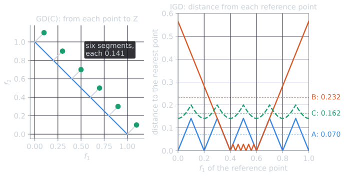
where $d_i$ is the Euclidean distance from $\mathbf{a}_i$ to the nearest reference point. The form usually quoted uses $p = 2$, and then the value depends on the number of points as well as their distances: six points each $0.141$ from the front give $0.141 / \sqrt{6} = 0.058$. Many later studies use $p = 1$, the plain mean of the $d_i$, which Ishibuchi et al. (2015) adopt because its meaning is clear. This article uses $p = 1$. Smaller is better, and zero means every point lies on the front.
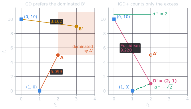
GD cannot see coverage. Fronts A, B, and D all have $\mathrm{GD} = 0$, although B covers a fifth of the front. Worse, GD can prefer a dominated set. Zitzler et al. (2003) gave the example of a front consisting of the two points $(1, 0)$ and $(0, 10)$, with approximation sets $A' = \{(2, 5)\}$ and $B' = \{(3, 9)\}$. The point $(2, 5)$ dominates $(3, 9)$, yet $(3, 9)$ is closer to $(0, 10)$ than $(2, 5)$ is to either reference point, so $\mathrm{GD}(A') = 5.099$ and $\mathrm{GD}(B') = 3.162$, and GD ranks the dominated set first.
Inverted generational distance and IGD+
Inverted generational distance (IGD) reverses the direction of measurement: the average distance from each reference point to the nearest point of $A$,
$$\mathrm{IGD}(A) = \frac{1}{k} \sum_{j=1}^{k} \min_{\mathbf{a} \in A} \lVert \mathbf{z}_j - \mathbf{a} \rVert.$$
Ishibuchi et al. (2015) trace the name to Coello Coello and Reyes Sierra (2004), and note that similar measures had been used earlier. Because every part of the front must find a nearby point, IGD penalizes gaps as well as distance. Front B, on the front but narrow, has $\mathrm{IGD} = 0.232$, the worst of the four, since reference points near either end of the front are far from its cluster. Split by where the reference point lies, the 40 reference points with $f_1 < 0.4$ contribute distances summing to 11.597, the largest being $0.4\sqrt{2} = 0.566$ from the end $(0, 1)$ to the cluster's first point $(0.4, 0.6)$; the 40 with $f_1 > 0.6$ contribute the same by symmetry; and the 21 inside the cluster contribute only 0.283 in total. The mean is $23.476 / 101 = 0.232$. Almost all of B's IGD comes from the parts of the front it does not cover. Ishibuchi et al. (2015) describe IGD as the indicator most frequently used in studies with many objectives, where the hypervolume is expensive. It inherits a dependence on $Z$: the indicator rewards approximating the reference set, so a sparse or unevenly sampled $Z$ distorts it.
GD for front C is the opposite case. Each point of C is the point of A moved by $(0.1, 0.1)$, straight away from the line $f_1 + f_2 = 1$, so its nearest reference point is the point of A it came from, at distance $0.1\sqrt{2} = 0.141$. All six distances are equal and $\mathrm{GD}(C) = 0.141$.
IGD is not Pareto compliant either. Adding $D' = \{(2, 1)\}$ to the example above, $D'$ dominates $A'$, but $\mathrm{IGD}(A') = 5.242$ and $\mathrm{IGD}(D') = 5.317$, because $(2, 1)$ is far from the reference point $(0, 10)$ (Ishibuchi et al., 2015). The remedy proposed by Ishibuchi et al. (2015), IGD+, changes the distance. Only the amounts by which a point is worse than the reference point count:
$$d^{+}(\mathbf{z}, \mathbf{a}) = \sqrt{\textstyle\sum_{i=1}^{m} \big(\max\{a_i - z_i, 0\}\big)^2 }.$$
A point that is better than $\mathbf{z}$ in some objective is not penalized for it. With this distance, $\mathrm{IGD^{+}}(D') = 1.707$, $\mathrm{IGD^{+}}(A') = 3.550$, and $\mathrm{IGD^{+}}(B') = 6.110$, in the order dominance requires.
The calculation for $D' = (2, 1)$ shows where the difference comes from. From the reference point $(0, 10)$, the Euclidean distance is $\sqrt{2^2 + 9^2} = 9.220$, but $D'$ is 9 better than $(0, 10)$ in $f_2$, and only its excess of 2 in $f_1$ counts under $d^{+}$, so $d^{+} = \sqrt{2^2 + 0^2} = 2$. From $(1, 0)$, $D'$ is worse in both objectives, by 1 each, and both distances are $\sqrt{2} = 1.414$. IGD averages $9.220$ and $1.414$ to get $5.317$; IGD+ averages $2$ and $1.414$ to get $1.707$. Ishibuchi et al. (2015) showed that IGD+ is weakly Pareto compliant: if $A$ is better than $B$, IGD+ never ranks $B$ ahead, though it may call them equal.
Spacing and spread
Two indicators measure only the distribution of the points. Spacing (Schott, 1995) is the standard deviation of each point's distance to its nearest neighbor, with distance measured in the $L_1$ norm:
$$\mathrm{SP}(A) = \sqrt{\frac{1}{n-1} \sum_{i=1}^{n} (\bar{d} - d_i)^2 }, \qquad d_i = \min_{j \ne i} \sum_{k=1}^{m} \lvert a_{ik} - a_{jk} \rvert,$$
where $\bar{d}$ is the mean of the $d_i$. Zero means perfectly even spacing. It says nothing about where the points are: A, B, and C all score zero, because each has equal gaps, and D scores $0.612$.
The spread $\Delta$ of Deb, Pratap, Agarwal, and Meyarivan (2002), introduced with NSGA-II, adds the extent of the front. For two objectives, sort the points by $f_1$, let $d_1, \dots, d_{n-1}$ be the Euclidean distances between consecutive points and $\bar{d}$ their mean, and let $d_f$ and $d_l$ be the distances from the two ends of the true front to the set's two boundary points:
$$\Delta = \frac{d_f + d_l + \sum_{i=1}^{n-1} \lvert d_i - \bar{d} \rvert}{d_f + d_l + (n-1)\,\bar{d}}.$$
$\Delta = 0$ for points spaced evenly from end to end. Deb et al. (2002) note that it can exceed 1, and it does for D, at $1.2$, because D's uneven gaps make the sum of deviations exceed the denominator's $(n-1)\bar{d}$ term. As written, $\Delta$ is defined for two objectives, where points can be ordered along the front.
The ε-indicator
The additive ε-indicator asks how far a set must be translated to weakly dominate another. Between two sets,
$$I_{\epsilon+}(A, B) = \max_{\mathbf{b} \in B} \; \min_{\mathbf{a} \in A} \; \max_{1 \le i \le m} (a_i - b_i),$$
the smallest $\epsilon$ such that every point of $B$ is weakly dominated by some point of $A$ moved by $-\epsilon$ in every objective. Zitzler et al. (2003) introduced it together with a multiplicative version, in which the shift is replaced by a factor. As a binary indicator it compares two sets directly. Used against the reference set, $I_{\epsilon+}(A, Z)$ becomes a unary indicator, and it too is weakly Pareto compliant (Ishibuchi et al., 2015). For front A it is 0.1: the reference point $(0.1, 0.9)$, halfway between two points of A, needs a shift of 0.1. For C it is 0.2, the shift of 0.1 plus the same gap.
The four fronts
| Front | HV | GD | IGD | IGD+ | $I_{\epsilon+}$ | SP | Δ |
|---|---|---|---|---|---|---|---|
| A, even | 0.610 | 0.000 | 0.070 | 0.050 | 0.100 | 0.000 | 0.000 |
| B, clustered | 0.466 | 0.000 | 0.232 | 0.164 | 0.400 | 0.000 | 0.800 |
| C, shifted | 0.400 | 0.141 | 0.162 | 0.162 | 0.200 | 0.000 | 0.167 |
| D, uneven | 0.385 | 0.000 | 0.227 | 0.161 | 0.400 | 0.612 | 1.200 |
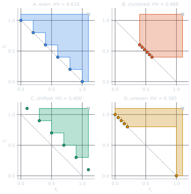
Every indicator puts A first or tied for first, as it should, since A is on the front, covers it, and is evenly spaced. Below A they part ways. Ranked from best to worst, the hypervolume gives B, C, D; IGD gives C, D, B; IGD+ gives D, C, B, by margins of a few thousandths; spacing calls A, B and C equal and D the worst; and GD calls A, B and D equal and C the worst.
The opening question, B against C, splits the indicators. The hypervolume, GD and spacing prefer B or call them equal: B lies on the front, and B's points, all close to the middle, dominate more area than C's, two of whose points sit on the boundary of the reference box and contribute nothing. IGD, IGD+, the ε-indicator and $\Delta$ prefer C, because C covers the whole front. None of these verdicts contradicts dominance, since B and C are incomparable. They express different preferences, and an indicator chosen after the results are in can make either algorithm the winner.
The script tools/experiments/evolution/indicators.py in the site repository computes every number in this article, and indicators_worked.py prints the intermediate values in the worked examples.
The demo below computes the hypervolume, GD and IGD of any set of points, with the same reference set and conventions. The presets are the fronts of this article. Some things to try: load B and drag its last point, (0.6, 0.4), along the front toward (1, 0): at $f_1 = 0.8$ the hypervolume has risen from 0.466 to 0.518 and IGD has fallen from 0.232 to 0.167, but at $(1, 0)$ both are worse again (0.490 and 0.185), because the point now leaves a gap behind it; add a point inside A's shaded region and see that it is drawn hollow and changes nothing, because it is dominated, while a point just behind the front but in one of the notches of the staircase, such as (0.1, 0.95), is non-dominated and raises the hypervolume; load P, which starts with the reference point at (1.0, 1.0), and switch on the exclusive contributions to see that its end points own nothing; then raise the reference point past 1.23 and compare with Q at the same reference point.
What unary indicators can and cannot say
Zitzler et al. (2003) gave these observations a formal footing. They asked what a comparison of indicator values can prove about the relation between two approximation sets, and proved the following.
- No unary indicator can decide "better". There is no unary indicator, and no finite combination of unary indicators, whose values can always show whether one approximation set is better than another. The obstacle is not the choice of indicators; any finite list of numbers loses information that the sets carry.
- "Not worse" is the best a unary indicator can prove. The hypervolume is the only unary indicator they knew of that detects, for every pair, that one set is not worse than another: a higher hypervolume rules out the lower set being better. Other indicators, including the unary ε-indicator, at best support the same "not worse" inference.
- Many indicators prove nothing about dominance. Diversity indicators, of which spacing and spread are examples, and distance indicators such as GD are neither compatible nor complete with respect to any dominance relation. A set may score better on all of them and still be dominated, as the set $\{(3, 9)\}$ scores better on GD than the set $\{(2, 5)\}$ that dominates it.
- Detecting dominance needs as many indicators as objectives. Even to tell whether one objective vector dominates another, a combination of unary indicators needs at least $m$ of them for $m$ objectives.
- Binary indicators avoid these limits. An indicator that takes two sets, such as the binary ε-indicator, can detect whether one set is better than another. The price is that the number of values grows with the square of the number of sets compared. For general statements Zitzler et al. (2003) recommend the binary ε-indicator.
Their analysis assumes a single run of each optimizer. With repeated runs, each indicator becomes a distribution of values, and comparisons need statistical tests over runs, the same issue that significance testing addresses in comparing retrieval systems. Reporting several indicators, chosen to match what a decision maker wants from the front, gives a fuller picture than any one of them. When the indicators disagree, the disagreement is information about the trade-offs between algorithms, not noise to be averaged away. Ranking optimizers with Pareto optimality describes one attempt to combine many indicators without weighting them, by treating the indicator values themselves as objectives.
References
- Bringmann, K., and Friedrich, T. (2010). Approximating the volume of unions and intersections of high-dimensional geometric objects. Computational Geometry, 43(6–7), 601–610.
- Coello Coello, C. A., and Reyes Sierra, M. (2004). A study of the parallelization of a coevolutionary multi-objective evolutionary algorithm. In MICAI 2004: Advances in Artificial Intelligence, Lecture Notes in Computer Science 2972, 688–697. Springer.
- Deb, K., Pratap, A., Agarwal, S., and Meyarivan, T. (2002). A fast and elitist multiobjective genetic algorithm: NSGA-II. IEEE Transactions on Evolutionary Computation, 6(2), 182–197.
- Ishibuchi, H., Imada, R., Setoguchi, Y., and Nojima, Y. (2018). How to specify a reference point in hypervolume calculation for fair performance comparison. Evolutionary Computation, 26(3), 411–440.
- Ishibuchi, H., Masuda, H., Tanigaki, Y., and Nojima, Y. (2015). Modified distance calculation in generational distance and inverted generational distance. In Evolutionary Multi-Criterion Optimization (EMO 2015), Lecture Notes in Computer Science 9019, 110–125. Springer.
- Lacour, R., Klamroth, K., and Fonseca, C. M. (2017). A box decomposition algorithm to compute the hypervolume indicator. Computers & Operations Research, 79, 347–360.
- Schott, J. R. (1995). Fault Tolerant Design Using Single and Multicriteria Genetic Algorithm Optimization. Master's thesis, Department of Aeronautics and Astronautics, Massachusetts Institute of Technology.
- Van Veldhuizen, D. A. (1999). Multiobjective Evolutionary Algorithms: Classifications, Analyses, and New Innovations. PhD dissertation, Air Force Institute of Technology.
- While, L., Bradstreet, L., and Barone, L. (2012). A fast way of calculating exact hypervolumes. IEEE Transactions on Evolutionary Computation, 16(1), 86–95.
- Zitzler, E., and Thiele, L. (1998). Multiobjective optimization using evolutionary algorithms: A comparative case study. In Parallel Problem Solving from Nature (PPSN V), Lecture Notes in Computer Science 1498, 292–301. Springer.
- Zitzler, E., and Thiele, L. (1999). Multiobjective evolutionary algorithms: A comparative case study and the strength Pareto approach. IEEE Transactions on Evolutionary Computation, 3(4), 257–271.
- Zitzler, E., Thiele, L., Laumanns, M., Fonseca, C. M., and Grunert da Fonseca, V. (2003). Performance assessment of multiobjective optimizers: An analysis and review. IEEE Transactions on Evolutionary Computation, 7(2), 117–132.