For the paper presentation in CSC 742 I chose "A Novel Pareto-optimal Ranking Method for Comparing Multi-objective Optimization Algorithms" by Amin Ibrahim, Azam Asilian Bidgoli, Shahryar Rahnamayan, and Kalyanmoy Deb, posted to arXiv in November 2024 (Ibrahim, Bidgoli, Rahnamayan, and Deb, 2024). The paper addresses a problem that the course's material on quality indicators leaves open. Each indicator reduces a front to one number, different indicators reward different properties, and they often rank the same algorithms differently. The paper's answer is to apply the idea at the center of multi-objective optimization to the evaluation itself: treat each indicator as an objective, and rank algorithms by Pareto dominance over their indicator scores.
The presentation followed the paper's structure: the motivation, the ten indicators the paper uses, the ranking procedure, its four ranking rules on the paper's small example, and the experiments on the 2018 CEC competition. This article covers the same ground from the paper itself, recomputes the paper's overall ranking from its published counts, and adds a small worked example of my own that shows where the method is sensitive.
The problem
A multi-objective optimizer returns a set of trade-offs, not a single value, so comparing two optimizers means comparing two sets. Quality indicators make the comparison numeric, and each captures some aspects of quality and misses others. Generational distance sees only closeness to the true front, spacing sees only evenness, the hypervolume combines several properties but depends on a reference point. Zitzler, Thiele, Laumanns, Fonseca, and Grunert da Fonseca (2003) proved that no finite set of unary indicators can, in general, establish that one approximation set is better than another. In practice studies report several indicators, and the rankings they imply can conflict.
Competitions need one ranking, so they combine indicators by a fixed rule. The 2018 CEC competition on many-objective optimization, whose data the paper uses, ranked the entries by the mean IGD and mean hypervolume on each problem, giving 90 rankings, and scored each algorithm by the sum of the reciprocals of its ranks (Ibrahim et al., 2024, Section V-E). The paper's argument is that two indicators capture too little, and that existing techniques for merging indicators into one score are hard to design without distorting the individual indicators, and combine only two or three of them.
The method
Suppose $A$ algorithms are compared on one test problem using $M$ indicators, with each algorithm run $R$ times. The procedure has six steps (Ibrahim et al., 2024, Section IV):
- Choose $M$ performance indicators.
- Run each algorithm $R$ times.
- Score every run on all $M$ indicators, giving an $R \times M$ matrix per algorithm.
- Stack the matrices into $A \times R$ points, each an $M$-dimensional vector of indicator values for one run.
- Apply non-dominated sorting to the $A \times R$ vectors, after converting every indicator to minimization; an indicator where larger is better, such as the hypervolume, is replaced by its reciprocal or its negative.
- Count how many of each algorithm's runs fall on each Pareto level, and rank the algorithms from these counts.
Step 5 is the non-dominated sorting used by NSGA-II (Deb, Pratap, Agarwal, and Meyarivan, 2002), applied to runs rather than to candidate solutions. Level 1 holds the runs whose indicator vectors no other run dominates; level 2 holds those dominated only by level-1 runs; and so on. Step 6 produces an $A \times L$ count matrix, where $L$ is the number of levels and each row sums to $R$. For several problems, the paper sorts each problem separately and adds the count matrices level by level, so that level 1 means "on the first level of its own problem".
The method at its smallest
Before the paper's own example, it helps to watch steps 3 to 6 on a case small enough to sort by hand. The case is mine, with numbers chosen to make a point rather than produced by any real optimizer. Two algorithms, X and Y, are each run four times, and each run is scored on two indicators, GD and IGD, both to be minimized. Step 4 stacks the eight runs into eight two-dimensional points:
| Run | GD | IGD | Dominated by | Level |
|---|---|---|---|---|
| $x_1$ | 0.02 | 0.20 | none | 1 |
| $x_2$ | 0.20 | 0.03 | none | 1 |
| $x_3$ | 0.30 | 0.30 | $x_1, x_2, y_1, y_2, y_3, y_4$ | 3 |
| $x_4$ | 0.40 | 0.45 | every other run | 4 |
| $y_1$ | 0.08 | 0.08 | none | 1 |
| $y_2$ | 0.10 | 0.12 | $y_1$ | 2 |
| $y_3$ | 0.12 | 0.10 | $y_1$ | 2 |
| $y_4$ | 0.09 | 0.15 | $y_1$ | 2 |
Step 5 sorts them. No run is better than $x_1$ on GD, none is better than $x_2$ on IGD, and nothing is better than $y_1$ on both, so these three are mutually non-dominated and form level 1. Removing them leaves $y_2$, $y_3$ and $y_4$ undominated: each is beaten only by $y_1$. They form level 2. Then $x_3$, which every Y run beats on both indicators, forms level 3, and $x_4$, worse than $x_3$ on both, forms level 4.
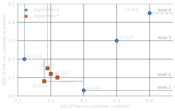
Step 6 counts each algorithm's runs per level:
| Level 1 | Level 2 | Level 3 | Level 4 | |
|---|---|---|---|---|
| X | 2 | 0 | 1 | 1 |
| Y | 1 | 3 | 0 | 0 |
X has more runs on the first level, and Y has no run below the second. Which is better depends on how the levels are weighed, and that is the job of the ranking rules. The section after next returns to X and Y with all four rules.
Four ranking rules
The count matrix must still be turned into a ranking. The paper's example has two algorithms, each with 31 runs:
| Level 1 | Level 2 | Level 3 | |
|---|---|---|---|
| $a_1$ | 20 | 10 | 1 |
| $a_2$ | 15 | 14 | 2 |
Olympic. Rank by the number of level-1 runs, like ordering countries by gold medals, and break ties with level 2, then level 3. Here $a_1$ wins, 20 to 15, although $a_2$ has more level-2 runs.
Linear. Weight level $l$ by $L - l + 1$, so with three levels the weights are 3, 2, 1, and rank by the weighted sum:
$$\text{Linear}(a_1) = 20 \cdot 3 + 10 \cdot 2 + 1 \cdot 1 = 81, \qquad \text{Linear}(a_2) = 15 \cdot 3 + 14 \cdot 2 + 2 \cdot 1 = 75.$$
Exponential. Weight level $l$ by $2^{-(l-1)}$, so each level counts half as much as the one above:
$$\text{Exp}(a_1) = 20 + 10 \cdot \tfrac{1}{2} + 1 \cdot \tfrac{1}{4} = 25.25, \qquad \text{Exp}(a_2) = 15 + 14 \cdot \tfrac{1}{2} + 2 \cdot \tfrac{1}{4} = 22.5.$$
The paper's prose lists the weights as $2^0, 2^{-1}, 2^{-3}, \dots$, but its equation and its example use $2^{-(l-1)}$, as here.
Adaptive. Let $CW(a, l)$ be the cumulative number of runs of algorithm $a$ on levels 1 to $l$, and $\mathrm{Total}(l)$ its sum over all algorithms. The score is each algorithm's share of the cumulative total, summed over levels:
$$\text{Adaptive}(a) = \sum_{l=1}^{L} \frac{CW(a, l)}{\mathrm{Total}(l)}.$$
The cumulative counts are $20, 30, 31$ for $a_1$ and $15, 29, 31$ for $a_2$, with totals $35, 59, 62$, so
$$\text{Adaptive}(a_1) = \tfrac{20}{35} + \tfrac{30}{59} + \tfrac{31}{62} = 1.58, \qquad \text{Adaptive}(a_2) = \tfrac{15}{35} + \tfrac{29}{59} + \tfrac{31}{62} = 1.42.$$
All four rules prefer $a_1$ here. They differ in how much the lower levels count: nothing unless there is a tie under the Olympic rule, a little under the exponential rule, and steadily under the linear rule.
When the rules disagree
The paper's example is one where every rule agrees. X and Y, from the small example above, are one where they do not. With $L = 4$ levels, the linear weights are 4, 3, 2, 1 and the exponential weights $1, \tfrac{1}{2}, \tfrac{1}{4}, \tfrac{1}{8}$. The cumulative counts are $2, 2, 3, 4$ for X and $1, 4, 4, 4$ for Y, with totals $3, 6, 7, 8$. Rounded to four decimals:
| Rule | X | Y | Winner |
|---|---|---|---|
| Olympic (level-1 count) | 2 | 1 | X |
| Linear | $2 \cdot 4 + 0 \cdot 3 + 1 \cdot 2 + 1 \cdot 1 = 11$ | $1 \cdot 4 + 3 \cdot 3 = 13$ | Y |
| Exponential | $2 + 0 + \tfrac{1}{4} + \tfrac{1}{8} = 2.375$ | $1 + \tfrac{3}{2} = 2.5$ | Y |
| Adaptive | $\tfrac{2}{3} + \tfrac{2}{6} + \tfrac{3}{7} + \tfrac{4}{8} = 1.9286$ | $\tfrac{1}{3} + \tfrac{4}{6} + \tfrac{4}{7} + \tfrac{4}{8} = 2.0714$ | Y |
The Olympic rule rewards X's two specialist runs and ignores everything else, since the level-1 counts differ. The other three rules see that half of X's runs are poor and prefer Y's consistency. The average of the four ranks, the paper's recommended summary, puts Y first: Y's mean rank is $(2 + 1 + 1 + 1)/4 = 1.25$ and X's is 1.75. The same tension decides the middle of the paper's overall ranking, as the experiments below show. The script tools/experiments/evolution/pareto_ranking.py computes this example in its part 4.
The paper presents the method as free of parameters and scalable, since any number of algorithms, runs, and indicators can be included without new settings, and as applicable to any setting where several metrics must be combined into one ranking.
The experiments
The paper ranks the ten algorithms entered in the 2018 IEEE CEC competition on many-objective optimization: AGE-II, AMPDEA, BCE-IBEA, CVEA3, fastCAR, HHcMOEA, KnEA, RPEA, RSEA, and RVEA. The problems were the 15 MaF benchmark problems (Cheng et al., 2017), with 5, 10, and 15 objectives, and every algorithm was run 20 times on each, with at most $\max(100{,}000, 10{,}000 \times D)$ evaluations for $D$ decision variables and a population of at most 240. Each run was scored on ten indicators: hypervolume, generational distance, IGD, two-set coverage, coverage over the Pareto front, the averaged Hausdorff distance $\Delta_p$, pure diversity, spacing, overall Pareto spread, and the distribution metric (Ibrahim et al., 2024, Section III).
One problem at a time. On 5-objective MaF1, sorting the 200 runs gave 7 levels. HHcMOEA had 19 of its 20 runs on level 1 and AGE-II 17, while RVEA's runs were scattered over all seven levels. On 15-objective MaF10, sorting gave 6 levels, and CVEA3 and HHcMOEA had all 20 runs on level 1. The rules mostly agreed, but not always: on 5-objective MaF1, AMPDEA was 10th by the Olympic rule and 9th by the other three. The counts show why: AMPDEA had the fewest level-1 runs, 4 against RVEA's 5, but none on the two lowest levels, where RVEA had 5. The Olympic rule also produced ties, such as three algorithms sharing first place on 15-objective MaF1.
One number of objectives at a time. Summing the counts over the 15 problems gives 300 runs per algorithm. At 10 objectives CVEA3 had the most level-1 runs, 274. At 15 objectives fastCAR had the most, 238, and ranked first under all four rules. HHcMOEA, with 232 level-1 runs, was second by the Olympic rule but sixth by the linear rule, because 40 of its runs sat on levels 6 to 12.
Overall. Summing over all 45 problem instances gives 900 runs per algorithm spread over at most 18 levels. FastCAR and HHcMOEA each had 747 runs on level 1; the Olympic rule separates them at level 2, where fastCAR had 83 and HHcMOEA 53.
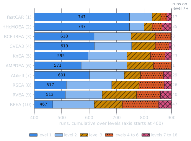
The overall ranks were:
| Rule | AGE-II | AMPDEA | BCE-IBEA | CVEA3 | fastCAR | HHcMOEA | KnEA | RPEA | RSEA | RVEA |
|---|---|---|---|---|---|---|---|---|---|---|
| Olympic | 5 | 7 | 4 | 3 | 1 | 2 | 6 | 10 | 8 | 9 |
| Linear | 7 | 5 | 2 | 4 | 1 | 3 | 6 | 10 | 8 | 9 |
| Exponential | 6 | 7 | 4 | 3 | 1 | 2 | 5 | 10 | 8 | 9 |
| Adaptive | 7 | 5 | 3 | 4 | 1 | 2 | 6 | 10 | 8 | 9 |
| Average | 7 | 6 | 3 | 4 | 1 | 2 | 5 | 10 | 8 | 9 |
The "Average" row ranks the algorithms by their mean rank under the four rules. Applying the four rules to the level counts in the paper's Table IV reproduces every entry of its Table V, shown here, and the 15-objective ranks of HHcMOEA quoted above. FastCAR is first under every rule and RPEA last; the middle of the table moves by up to two places between rules. The paper reports average pairwise correlations between the rules' rankings of 0.947 for Olympic, 0.923 for linear, 0.956 for exponential, and 0.960 for adaptive. It recommends the average rank across the four rules, or the adaptive rule when only one is wanted, mainly because the adaptive ranking agreed most closely with the other three.
Against the competition. To compare like with like, the paper also ranked the algorithms using only the hypervolume and IGD, the competition's two indicators:
| AGE-II | AMPDEA | BCE-IBEA | CVEA3 | fastCAR | HHcMOEA | KnEA | RPEA | RSEA | RVEA | |
|---|---|---|---|---|---|---|---|---|---|---|
| Competition (HV and IGD) | 5 | 2 | 3 | 1 | 6 | 8 | 7 | 10 | 4 | 9 |
| Method, HV and IGD, average rank | 4 | 2 | 3 | 1 | 5 | 9 | 7 | 10 | 5 | 8 |
| Method, ten indicators, average rank | 7 | 6 | 3 | 4 | 1 | 2 | 5 | 10 | 8 | 9 |
With the same two indicators, the method and the competition agree closely: CVEA3 first, AMPDEA second, RPEA last, and no algorithm more than one place apart. With ten indicators the picture changes. FastCAR moves from sixth to first, HHcMOEA from eighth to second, and AMPDEA from second to sixth. The paper reads this as evidence that two indicators miss aspects of performance that the other eight capture.
Limitations
The paper names two limitations itself. The ranking depends on which indicators are chosen, and they should be chosen to match the goal of the comparison. And the method could be exploited by an algorithm customized to excel on one indicator, which would then reach the top under Pareto dominance; a run that is strictly best on any single indicator cannot be dominated. As a remedy, the paper suggests replacing Pareto dominance with a relation it calls ε-dominance, taken from Kang et al. (2007): one run dominates another if it is better on more indicators than it is worse on, and its vector of indicator values has the smaller norm.
Several further points follow from the definitions, and are my own observations rather than the paper's:
- More indicators mean coarser levels. With ten indicators, a run is dominated only if another run is at least as good on all ten, which becomes less likely with every indicator added. Summing the paper's Table IV, 5,995 of the 9,000 runs, two thirds, sit on level 1 of their problem. The rankings are decided largely by how many runs fall off level 1, not by the order among the runs that stay on it.
- No account of uncertainty. The method produces ranks but no measure of how likely they are to change with another 20 runs. A difference of a few level-1 runs between two algorithms may not be meaningful, and the paper does not test it. Indicator values over repeated runs are samples, and comparing them calls for the kind of tests discussed in significance testing.
- Indicators that overlap. The ten indicators are not independent. The averaged Hausdorff distance $\Delta_p$, as the paper defines it, is the larger of GD and IGD, and the paper classes five of the ten as measuring diversity alone. Pareto dominance gives no weights, but the choice of which aspects to measure, and how many times, acts as one.
- A constant term. In the adaptive score, the last term is the same for every algorithm, since every algorithm has all $R$ of its runs on some level: $R / (A R) = 1 / A$. In the paper's example it is $31/62$ for both. It shifts the scores without affecting the ranks.
- A binary indicator as a unary score. Two-set coverage $C(A, B)$ compares two sets, and the paper does not say how it was reduced to one value per run.
- Level counts across problems. Adding counts level by level treats level 2 of a problem with 3 levels the same as level 2 of a problem with 12, although the first is close to the bottom and the second close to the top.
A worked example
To see the method at work on a case where the answer is known, the script tools/experiments/evolution/pareto_ranking.py in the site repository creates five hypothetical algorithms on a two-objective problem whose true front is the line $f_1 + f_2 = 1$. Each run produces ten points of the form $(x + o, 1 - x + o)$, a point on the front at $f_1 = x$ moved back by $o$ in both objectives, keeps the non-dominated ones, and is scored on five indicators from quality indicators for Pareto fronts: hypervolume with reference point $(1.1, 1.1)$, GD, IGD, spacing, and the spread $\Delta$. Each algorithm is run ten times, with the random generator seeded at 2024. The five generators are:
- Narrow: $x$ uniform on a random window of width 0.3, $o = \lvert N(0, 0.005) \rvert$; close to the front but covering a third of it.
- Wide: $x$ evenly spaced from 0 to 1 with $N(0, 0.02)$ jitter, clipped to $[0, 1]$, $o = 0.06 + \lvert N(0, 0.02) \rvert$; even coverage, well behind the front.
- Random: $x$ uniform on $[0, 1]$, $o = \lvert N(0, 0.02) \rvert$; close and covering the front, unevenly spaced.
- Erratic: $x$ evenly spaced with $N(0, 0.01)$ jitter; on each run, with probability one half, $o = 0.005 + \lvert N(0, 0.005) \rvert$, otherwise $o = 0.12 + \lvert N(0, 0.005) \rvert$.
- Weak: $x$ uniform on $[0.2, 0.8]$, $o = 0.10 + \lvert N(0, 0.02) \rvert$; behind the front and covering its middle.
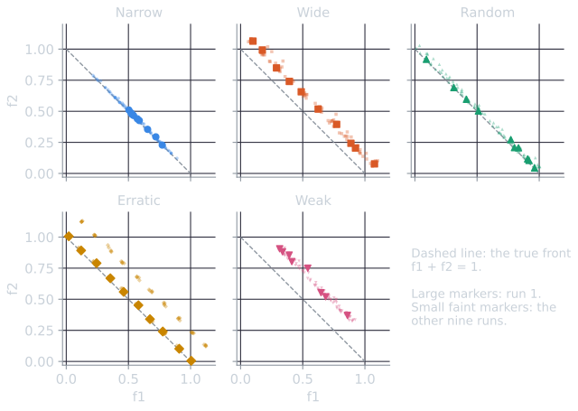
The median indicator values over the ten runs were:
| HV | GD | IGD | SP | Δ | |
|---|---|---|---|---|---|
| Narrow | 0.4605 | 0.0063 | 0.2384 | 0.0342 | 0.9033 |
| Wide | 0.4958 | 0.1044 | 0.1142 | 0.0377 | 0.2993 |
| Random | 0.5860 | 0.0215 | 0.0717 | 0.0908 | 0.6694 |
| Erratic | 0.5173 | 0.0945 | 0.1118 | 0.0196 | 0.2191 |
| Weak | 0.3898 | 0.1619 | 0.2082 | 0.0532 | 0.7746 |
Random has the best hypervolume and IGD, the two indicators that combine closeness and coverage. Non-dominated sorting of the 50 runs on all five indicators gave six levels:
| L1 | L2 | L3 | L4 | L5 | L6 | |
|---|---|---|---|---|---|---|
| Narrow | 4 | 6 | 0 | 0 | 0 | 0 |
| Wide | 0 | 3 | 3 | 2 | 2 | 0 |
| Random | 0 | 0 | 3 | 6 | 1 | 0 |
| Erratic | 2 | 3 | 3 | 2 | 0 | 0 |
| Weak | 0 | 0 | 1 | 2 | 5 | 2 |
With six levels, the linear weights run from 6 down to 1. The scores, with the exponential and adaptive ones rounded to four decimals, are:
| Linear | Exponential | Adaptive | |
|---|---|---|---|
| Narrow | 54 | 7.0000 | 2.2377 |
| Erratic | 45 | 4.5000 | 1.5552 |
| Wide | 37 | 2.6250 | 0.9893 |
| Random | 32 | 1.5625 | 0.7405 |
| Weak | 22 | 0.8750 | 0.4774 |
All four rules agree on Narrow, Erratic, Wide, Random, Weak, in that order. Ranking by each indicator alone, using the mean over the ten runs as the competition did, gives quite different orders:
| Ranked by | Narrow | Wide | Random | Erratic | Weak |
|---|---|---|---|---|---|
| Pareto-optimal method (all rules) | 1 | 3 | 4 | 2 | 5 |
| HV | 4 | 3 | 1 | 2 | 5 |
| GD | 1 | 4 | 2 | 3 | 5 |
| IGD | 5 | 3 | 1 | 2 | 4 |
| SP | 2 | 3 | 5 | 1 | 4 |
| Δ | 5 | 2 | 3 | 1 | 4 |
The method puts Narrow first, although Narrow is worst on IGD and Δ and fourth on hypervolume. The reason is GD. Narrow's largest GD over its ten runs, 0.0081, is smaller than the smallest GD of any run by any other algorithm, 0.0121. A run of another algorithm can dominate a Narrow run only by being no worse on every indicator, including GD, so no Narrow run is dominated by another algorithm's run, and every one of them sits on level 1 or 2, where only other Narrow runs dominate it. This is the exploit the paper warns of, produced here without any tuning, by an algorithm that simply converges to a small part of the front. Removing GD and sorting on the other four indicators moves Narrow to third and Erratic to first, under all four rules.
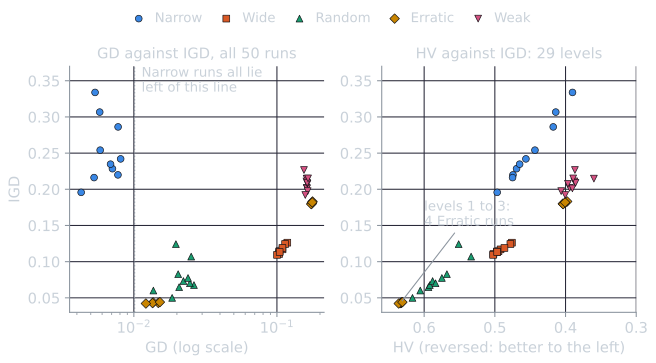
Random, the best algorithm by the two indicators that measure closeness and coverage together, ranks fourth. Every one of its ten runs is dominated by at least one of Erratic's runs, which is better on all five indicators at once; Erratic's own five poor runs are in turn dominated by runs of Wide. With only the hypervolume and IGD, the competition's two indicators, the sort gives 29 levels, nearly a total order of the 50 runs. Random then rises to second under three rules, behind Erratic, and to first under the linear rule.
The example illustrates the method's character rather than refuting it. The Pareto-optimal ranking rewards being excellent in some respect, measured by some indicator, and the indicators chosen define the respects. That is its intended behavior, and it means that the choice of indicators carries the weight that explicit weights would otherwise carry.
References
- Cheng, R., Li, M., Tian, Y., Zhang, X., Yang, S., Jin, Y., and Yao, X. (2017). A benchmark test suite for evolutionary many-objective optimization. Complex & Intelligent Systems, 3(1), 67–81.
- Deb, K., Pratap, A., Agarwal, S., and Meyarivan, T. (2002). A fast and elitist multiobjective genetic algorithm: NSGA-II. IEEE Transactions on Evolutionary Computation, 6(2), 182–197.
- Ibrahim, A., Bidgoli, A. A., Rahnamayan, S., and Deb, K. (2024). A novel Pareto-optimal ranking method for comparing multi-objective optimization algorithms. arXiv preprint arXiv:2411.17999.
- Kang, Z., Kang, L., Zou, X., Liu, M., Li, C., Yang, M., Li, Y., Chen, Y., and Zeng, S. (2007). A new evolutionary decision theory for many-objective optimization problems. In Advances in Computation and Intelligence (ISICA 2007), Lecture Notes in Computer Science 4683, 1–11. Springer.
- Zitzler, E., Thiele, L., Laumanns, M., Fonseca, C. M., and Grunert da Fonseca, V. (2003). Performance assessment of multiobjective optimizers: An analysis and review. IEEE Transactions on Evolutionary Computation, 7(2), 117–132.