The K-means algorithm is fully specified once three things are fixed: the starting centroids, the number of clusters $K$, and the vectors being clustered. The algorithm makes none of these choices itself, and each one changes the result. This article covers them in turn and measures their effect on a real collection.
The experiment
The test collection is the Reuters-21578 newswire collection (Lewis, 1997) used in text classification, restricted to stories with exactly one category from six: earn (earnings reports), acq (acquisitions), crude (oil), trade, money-fx (currency markets), and interest (interest rates). That leaves 7,487 stories, from the training and test portions together. The categories are very unequal in size: 3,918 earn stories and 2,292 acq, against 271 to 373 for each of the other four.
Each story was lowercased, split into alphabetic tokens, filtered against a short stop list, and stemmed with the Porter stemmer. Tokens of one letter were dropped. The 3,000 most widespread terms appearing in at least three stories became the features, weighted by TF-IDF with logarithmic term frequency and normalized to unit length. On unit vectors, squared Euclidean distance is $2 - 2\cos\theta$, so K-means distances follow cosine similarity.
The categories play no part in the clustering. They are used afterward to judge it, with purity, normalized mutual information (NMI), and the Rand index (RI), which evaluating clusterings defines. All three range from 0 to 1, higher meaning closer agreement with the categories.
Starting centroids and restarts
K-means converges to a local minimum of the residual sum of squares (RSS), and which minimum it reaches depends on where it starts. The simplest initialization picks $K$ documents at random as the starting centroids. Running it ten times with $K = 6$, each from a different random start:
| Measure | Lowest of 10 runs | Highest of 10 runs |
|---|---|---|
| RSS | 6,532.6 | 6,594.5 |
| Purity | 0.703 | 0.804 |
| NMI | 0.372 | 0.496 |
| Rand index | 0.659 | 0.721 |
| Iterations to converge | 16 | 69 |
RSS varies by only about one percent, but the clusterings differ a great deal. Purity ranges over ten points and NMI over twelve. Many quite different partitions of the collection have nearly the same RSS, and the starting point decides which one is found.
The standard remedy is restarts: run K-means several times and keep the result with the lowest RSS. This is sound, since RSS is the quantity K-means is trying to minimize and the only one available when there are no labels. It does not guarantee the clustering a person would prefer. Of the ten random runs, the one with the lowest RSS had purity 0.788, good but not the best of the ten.
k-means++
Random starting points can fall close together, in one dense region, leaving other regions without a centroid. k-means++ (Arthur and Vassilvitskii, 2007) spreads them out. It picks the first centroid uniformly at random. Each later centroid is chosen at random with probability proportional to $D(x)^2$, the squared distance from a document $x$ to the nearest centroid already chosen:
$$P(x \text{ is chosen next}) = \frac{D(x)^2}{\sum_{x'} D(x')^2}.$$
Points far from all existing centroids are therefore likely to be picked, and a point that is already a centroid has $D(x) = 0$ and cannot be picked again. Arthur and Vassilvitskii (2007, Theorem 3.1) proved that the expected RSS of this seeding alone, before any K-means iterations, is at most $8(\ln K + 2)$ times the optimum, a guarantee random initialization lacks; the iterations that follow can only lower it.
k-means++ on the small examples
The K-means algorithm gives two small cases where the starting points decide the outcome, and k-means++ can be worked out exactly on both.
The rectangle. Four points at $(0, 0)$, $(0, 2)$, $(6, 0)$ and $(6, 2)$, with $K = 2$. K-means ends in the bad top-and-bottom clustering (RSS 36, against 4 for the left-and-right one) exactly when both seeds are on the same side. Random seeding picks two of the four points, and 2 of the 6 possible pairs are on the same side, so it fails with probability $1/3$. With k-means++, suppose the first seed is $(0, 0)$. The squared distances to the other points are
| Candidate | $(0, 2)$ | $(6, 0)$ | $(6, 2)$ | Total |
|---|---|---|---|---|
| $D(x)^2$ | 4 | 36 | 40 | 80 |
| Probability | 0.05 | 0.45 | 0.50 | 1 |
so the second seed lands on the same side with probability $4/80 = 0.05$. By symmetry the same holds whichever corner comes first, and k-means++ fails with probability 0.05 instead of 0.33. Making the rectangle wider makes the bad clustering worse and k-means++ less likely to fall into it: with width $w$ and height 2, the failure probability is $4/(8 + 2w^2)$, which shrinks as the bad clustering's RSS, $w^2$, grows. That is the idea behind the guarantee: the seeding is most careful exactly where a mistake would cost most.
The six points. On the six points $A$ to $F$ of that article, 7 of the 15 seed pairs lead to the optimum (RSS 7.875) and 8 to the local minimum $\{A, B, C\}$, $\{D, E, F\}$ (RSS 10.67), so random seeding succeeds with probability $7/15 = 0.47$. Working through the $D^2$ probabilities for each of the six possible first seeds gives a success probability of 0.54 for k-means++, only a little better. Here the two outcomes have similar RSS, and both kinds of seed pair are spread out, so spreading the seeds does not separate good starts from bad ones. k-means++ protects against seeds bunched in one group, not against every poor start.
Ten runs on Reuters
The same ten runs with k-means++ seeding:
| Measure | Lowest of 10 runs | Highest of 10 runs |
|---|---|---|
| RSS | 6,528.7 | 6,582.7 |
| Purity | 0.713 | 0.839 |
| NMI | 0.352 | 0.586 |
| Rand index | 0.652 | 0.778 |
| Iterations to converge | 15 | 54 |
In these ten runs k-means++ found a slightly lower RSS, both at best and at worst, and needed at most 54 iterations against 69. Its range of purity and NMI was, if anything, wider. Its lowest-RSS run had purity 0.745, NMI 0.382, and RI 0.652, lower on all three than the lowest-RSS random run. Ten runs are too few to say whether those differences are real, which the next section tests with more.
Thirty seeds: seeding and restarts measured
The comparison above rests on ten runs of each kind, and the extremes of ten runs are noisy. Repeating it with 30 seeds for each seeding method, and reporting the median and interquartile range (the middle half of the 30 values), rounded as shown:
| Measure | Random seeds | k-means++ |
|---|---|---|
| RSS | 6,559 (6,549 to 6,575) | 6,571 (6,563 to 6,583) |
| Purity | 0.784 (0.740 to 0.802) | 0.782 (0.742 to 0.828) |
| NMI | 0.459 (0.401 to 0.509) | 0.486 (0.433 to 0.553) |
| Rand index | 0.703 (0.662 to 0.737) | 0.730 (0.700 to 0.763) |
| Adjusted Rand index | 0.305 (0.215 to 0.395) | 0.374 (0.301 to 0.455) |
| Iterations | 28.5 (21 to 39) | 26.5 (21 to 47) |
On this collection, k-means++ does not find tighter clusterings than random seeding. Its median RSS over these 30 runs is slightly higher, and over a larger set of 150 runs of each kind the two RSS distributions are practically identical (medians 6,567 and 6,568, and a Mann-Whitney test finds no difference, $p = 0.70$). Both methods reached the same lowest RSS, 6,526.9, in some run. The guarantee of Arthur and Vassilvitskii bounds how bad the seeding can be in expectation; it does not promise an improvement on a collection where random seeds already do well, as they evidently do here with six clusters and categories of very unequal size. What k-means++ did change here is the kind of local minimum found: its median NMI and adjusted Rand index are higher, so its clusterings agree somewhat better with the categories at the same RSS.
Restarts were measured the same way. For each of 30 replicates, K-means was run $r$ times from different seeds and the lowest-RSS result kept:
| Seeding | Restarts $r$ | RSS | NMI | Adjusted Rand |
|---|---|---|---|---|
| Random | 1 | 6,559 (6,549 to 6,575) | 0.459 (0.401 to 0.509) | 0.305 (0.215 to 0.395) |
| Random | 3 | 6,548 (6,533 to 6,554) | 0.425 (0.397 to 0.490) | 0.276 (0.205 to 0.335) |
| Random | 5 | 6,544 (6,533 to 6,550) | 0.425 (0.397 to 0.479) | 0.273 (0.205 to 0.328) |
| k-means++ | 1 | 6,571 (6,563 to 6,583) | 0.486 (0.433 to 0.553) | 0.374 (0.301 to 0.455) |
| k-means++ | 3 | 6,549 (6,541 to 6,556) | 0.457 (0.404 to 0.503) | 0.294 (0.243 to 0.365) |
| k-means++ | 5 | 6,542 (6,533 to 6,547) | 0.435 (0.397 to 0.474) | 0.286 (0.207 to 0.341) |
Restarts do their job: keeping the best of five runs lowers the median RSS by about 15 to 30 and narrows its spread. But agreement with the categories goes the other way. With either seeding, the best of five has lower NMI and adjusted Rand index than a single run. On Reuters the lowest-RSS clusterings are the ones that split the large earn category into several tight groups and merge the small categories, so minimizing RSS harder moves the result away from the editors' categories. Across all 300 runs, RSS and NMI are positively correlated (Spearman's $\rho = 0.30$): a worse RSS goes with a better match to the labels.
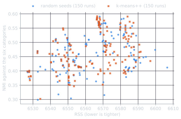
None of this makes restarts or k-means++ a mistake. Without labels, RSS is the only guide, and both reliably find low-RSS clusterings. The experiment shows what that objective means on a particular collection: tight clusters, not necessarily the categories a person had in mind.
What K-means found
The lowest-RSS k-means++ clustering, as a contingency table of clusters against categories:
| Cluster | earn | acq | crude | trade | money-fx | interest |
|---|---|---|---|---|---|---|
| 1 | 412 | 2,070 | 94 | 0 | 2 | 3 |
| 2 | 515 | 0 | 0 | 0 | 0 | 0 |
| 3 | 836 | 0 | 0 | 0 | 0 | 0 |
| 4 | 863 | 1 | 0 | 0 | 0 | 0 |
| 5 | 513 | 0 | 0 | 0 | 0 | 0 |
| 6 | 779 | 221 | 279 | 326 | 305 | 268 |
K-means divided earn into four nearly pure clusters and put all of trade, nearly all of money-fx and interest, and three quarters of crude together in one. The highest-weighted terms of each centroid show why. The four earn clusters are dividend announcements (qtly, div, payout), results reporting a loss, and two kinds of results tables, one marked by st and qtr (from "1st qtr", once the digits are stripped) and one by nine and mth (nine-month figures). These are formulaic notices with distinctive vocabularies, which K-means separates easily. The mixed cluster's top terms are rate, billion, bank, trade, and market, the shared language of economic news.
From K-means's point of view, this is a good clustering. Here, splitting a large, internally varied category lowered RSS more than separating four small categories with overlapping vocabulary. The clusters are coherent. They are just not the categories the Reuters editors chose. This is the general difficulty of judging a clustering against labels, taken up in evaluating clusterings.
Choosing K
K-means needs $K$ in advance, and RSS cannot choose it directly, because RSS always falls as $K$ grows. With $K = N$, every document is its own cluster and RSS is zero. The lowest RSS found in five k-means++ runs for each $K$:
| K | 2 | 3 | 4 | 5 | 6 | 8 | 10 | 12 | 15 | 20 |
|---|---|---|---|---|---|---|---|---|---|---|
| RSS | 6,848 | 6,684 | 6,639 | 6,591 | 6,529 | 6,474 | 6,399 | 6,354 | 6,284 | 6,199 |
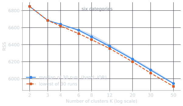
Repeating this with 30 k-means++ runs for each $K$ from 2 to 50 shows the whole curve and how much it varies from run to run. With two or three clusters all 30 runs found the same clustering; from four clusters on, the runs spread out, and the lowest of 30 runs is 20 to 40 below the median.
Two approaches are common (Manning, Raghavan, and Schütze, 2008, §16.4.1):
- Look for a knee. Plot RSS against $K$ and choose the point after which adding clusters helps much less. Here the largest drop is from two clusters to three. After that, RSS falls by roughly 15 to 60 per added cluster with no clear knee, and nothing in the curve points to six, the number of categories.
- Penalize complexity. Choose the $K$ that minimizes $\mathrm{RSS}(K) + \lambda K$, where the penalty $\lambda$ charges for each additional cluster. The Akaike information criterion gives one principled choice, $\lambda = 2M$ for $M$ dimensions. With $M = 3{,}000$ that penalty is 6,000 per cluster, far more than any drop in the table, so AIC would choose the smallest $K$ here. The general difficulty is that the answer depends on $\lambda$, which moves the choice of $K$ to a choice of $\lambda$.
With labels available, the external measures can be plotted against $K$ as well, and on Reuters the adjusted Rand index peaks at $K = 6$, the number of categories (evaluating clusterings shows the curves). But labels are exactly what clustering usually lacks, and a measure that needs them cannot choose $K$ for an unlabeled collection.
In practice $K$ is often set by the application. A search result clustering interface has room for perhaps five to ten clusters, and a browsing hierarchy for a manageable number of branches at each level.
Feature scaling
K-means uses Euclidean distance, which adds up squared differences in each feature. A feature measured in large units therefore outweighs one measured in small units, regardless of which matters more. TF-IDF vectors mostly avoid the problem. Every coordinate is a term weight in the same units, the differences in scale that IDF introduces are intended, and length normalization removes differences in document length. Clustering other kinds of objects, described by features in different units, usually requires standardizing each feature, subtracting its mean and dividing by its standard deviation, so that each has the same spread.
The Goodreads reviewer clustering shows what happens otherwise. Its features were average review length, as recorded in the dataset (most likely in characters), with values in the thousands, and three features on scales of a few units to about ten. Length accounted for more than 99.99 percent of the distances, and the clusters became bands of review length.
Spherical K-means
For text, what matters is usually the direction of a document vector, not its length. Standard K-means on unit vectors produces centroids that are shorter than unit length, since the mean of unit vectors pointing in different directions is shorter than any of them. Spherical K-means (Dhillon and Modha, 2001) normalizes each centroid back to unit length after the update step and assigns documents by cosine similarity to the centroids. It maximizes the total cosine similarity between documents and their centroids. Standard K-means on unit vectors assigns a document by its Euclidean distance to centroids of varying length, which is not the same as assigning by cosine, so the two can produce different clusterings.
A two-dimensional example shows how much shorter centroids get and why it matters. The mean of two orthogonal unit vectors, $(1, 0)$ and $(0, 1)$, is $(0.5, 0.5)$, of length $0.707$; a cluster whose members point in many directions has a centroid shorter still. For a unit document $\vec{x}$ and a centroid $\vec{\mu}$ at angle $\theta$,
$$\lvert \vec{x} - \vec{\mu} \rvert^2 = 1 + \lvert \vec{\mu} \rvert^2 - 2 \lvert \vec{\mu} \rvert \cos\theta,$$
which depends on the centroid's length as well as its direction. Take $\vec{x} = (1, 0)$, a short centroid $\vec{\mu}_1 = (0.3, 0)$ pointing exactly along it, and a unit-length centroid $\vec{\mu}_2$ at 35°. By cosine, $\vec{\mu}_1$ is the better match, 1 against 0.819. By squared distance, $\vec{\mu}_2$ is nearer, 0.362 against 0.490 (rounded to three decimals). Standard K-means sends the document to $\vec{\mu}_2$, and spherical K-means to $\vec{\mu}_1$. In general, standard K-means on text favors the tight clusters, whose centroids are long, over loose ones pointing the same way.
Summary
- Run K-means several times and keep the lowest RSS, but expect clusterings with similar RSS to differ substantially.
- k-means++ seeding guards against seeds bunched in one region, at almost no cost, and is the default in widely used libraries such as scikit-learn. On Reuters it did not lower RSS compared with random seeds, but it found clusterings closer to the categories.
- Keeping the lowest RSS of several runs lowers RSS reliably; on Reuters it also lowered agreement with the categories.
- RSS always decreases with $K$, so $K$ must come from a knee, a penalty, or the application.
- Put features on comparable scales before clustering, or the largest one will decide the result.
- K-means minimizes RSS, and on real collections that can mean splitting large categories and merging small ones.
The experiment scripts are tools/experiments/clustering/reuters_kmeans.py (the ten-run tables, the contingency table and RSS by $K$) and reuters_restarts.py (the 30-seed measurements), and the small examples are computed by lloyd_worked.py, all in the site repository.
References
- Arthur, D., and Vassilvitskii, S. (2007). k-means++: The advantages of careful seeding. In Proceedings of the Eighteenth Annual ACM-SIAM Symposium on Discrete Algorithms (SODA), 1027–1035.
- Dhillon, I. S., and Modha, D. S. (2001). Concept decompositions for large sparse text data using clustering. Machine Learning, 42(1–2), 143–175.
- Lewis, D. D. (1997). Reuters-21578 text categorization test collection, distribution 1.0.
- Manning, C. D., Raghavan, P., and Schütze, H. (2008). Introduction to Information Retrieval, section 16.4. Cambridge University Press.