Naive Bayes is the classifier most text classification courses teach first. It is derived in a few lines from Bayes' rule, it trains in a single pass over the data, it handles tens of thousands of features without difficulty, and it is often more accurate than its assumptions would suggest. On the ten largest categories of the Reuters-21578 news collection, the version built in this article reaches a micro-averaged F1 of 0.835. It rests on the same conditional independence assumption as the Binary Independence Model: the terms of a document are treated as independent of one another once the class is known. This article derives the classifier, explains how its probabilities are estimated and why, and carries the textbook's four-document example through every step, following Manning, Raghavan, and Schütze (2008, §13.2). The probability primer covers the background.
The running example
Manning, Raghavan, and Schütze (2008, §13.2) use four training documents, three in class China ($c$) and one not ($\bar{c}$, labeled Japan below), and one test document:
| Document | Text | Class |
|---|---|---|
| 1 | Chinese Beijing Chinese | China |
| 2 | Chinese Chinese Shanghai | China |
| 3 | Chinese Macao | China |
| 4 | Tokyo Japan Chinese | Japan |
| test | Chinese Chinese Chinese Tokyo Japan | ? |
The test document is ambiguous on purpose. It mentions Chinese three times, which points to China, but it also contains Tokyo and Japan, which have only ever appeared in the Japan document. Every section below computes something on this example, and all the numbers come from a script (tools/experiments/reuters/china_japan.py), rounded to three decimals unless stated.
From Bayes' rule to a classifier
The probability that document $d$ belongs to class $c$ follows from Bayes' rule:
$$P(c \mid d) = \frac{P(d \mid c)\, P(c)}{P(d)}.$$
To classify, choose the class with the highest posterior probability, the maximum a posteriori (MAP) class. $P(d)$ is the same for every class, so it can be dropped:
$$c_{\text{map}} = \arg\max_{c \in \mathbb{C}} P(d \mid c)\, P(c).$$
$P(c)$, the prior, is how common the class is. $P(d \mid c)$ is the probability of seeing this document if it belongs to class $c$, and estimating it is the difficulty. A document is a sequence of tokens $\langle t_1, t_2, \dots, t_{n_d} \rangle$, and there are far too many possible sequences to estimate their probabilities directly. Even the five-token test document is one of $6^5 = 7{,}776$ sequences over a six-term vocabulary, and the training set contains none of them. A model is needed that assigns a probability to a sequence it has never seen.
The generative story
Naive Bayes supplies that model by imagining how a document of class $c$ might have been written (Manning, Raghavan, and Schütze, 2008, §13.4):
- Choose the class $c$, with probability $P(c)$.
- Choose a length $n_d$.
- For each position $k = 1, \dots, n_d$, draw a term $t_k$ from the class's distribution over the vocabulary, $P(t \mid c)$, independently of every other position.
No one believes documents are written this way. The story is useful because it names exactly what the model must estimate: one prior per class and one distribution over the vocabulary per class. Under it, the probability of a particular document is
$$P(d \mid c) = P(n_d) \prod_{k=1}^{n_d} P(t_k \mid c).$$
The length term $P(n_d)$ is assumed to be the same for every class, so like $P(d)$ it cannot change which class wins, and it is dropped. Two assumptions are packed into step 3. Conditional independence: given the class, each token tells nothing about any other. Positional independence: the distribution is the same at every position, so word order is irrelevant and the document might as well be a bag of words. This is the multinomial model. A term occurring three times contributes its probability three times. The assumption is false, since Hong makes Kong far more likely, and word order matters. It is the same assumption the BIM makes, and it is "naive" for the same reason. Lewis (1998) traced the assumption's long history in retrieval and classification, where it has been used since the 1960s. Why the classifier works well anyway is the subject of the Bernoulli model and why Naive Bayes works.
The classifier becomes
$$c_{\text{map}} = \arg\max_{c} \; P(c) \prod_{k=1}^{n_d} P(t_k \mid c).$$
Estimating the parameters
The parameters are estimated from the training set by relative frequencies:
$$\hat{P}(c) = \frac{N_c}{N}, \qquad \hat{P}(t \mid c) = \frac{T_{ct}}{\sum_{t' \in V} T_{ct'}},$$
where $N_c$ is the number of training documents in class $c$, $N$ the total number of training documents, and $T_{ct}$ the number of occurrences of term $t$ in the training documents of class $c$, counting repeats.
Why relative frequencies
These are the maximum likelihood estimates: the values that make the training data most probable under the generative story. The derivation for the term probabilities is short. Write $\theta_t = P(t \mid c)$ for one class. Concatenate all of that class's training documents. Each occurrence of $t$ contributes a factor $\theta_t$, so the probability of the training tokens is $\prod_{t} \theta_t^{T_{ct}}$, and its logarithm is
$$\ell(\theta) = \sum_{t \in V} T_{ct} \log \theta_t.$$
The $\theta_t$ must form a probability distribution, $\sum_t \theta_t = 1$, so maximize with a Lagrange multiplier $\lambda$:
$$\frac{\partial}{\partial \theta_t} \Big[ \sum_{t'} T_{ct'} \log \theta_{t'} - \lambda \big( {\textstyle\sum_{t'}} \, \theta_{t'} - 1 \big) \Big] = \frac{T_{ct}}{\theta_t} - \lambda = 0 \quad\Longrightarrow\quad \theta_t = \frac{T_{ct}}{\lambda}.$$
Every $\theta_t$ is proportional to its count. Summing over $t$ and using the constraint gives $\lambda = \sum_{t'} T_{ct'}$, which is the relative frequency above. The same argument applied to the class labels gives $\hat{P}(c) = N_c / N$.
On the running example, the counts are:
| Term | $T_{ct}$, China | $T_{ct}$, Japan |
|---|---|---|
| Chinese | 5 | 1 |
| Beijing | 1 | 0 |
| Shanghai | 1 | 0 |
| Macao | 1 | 0 |
| Tokyo | 0 | 1 |
| Japan | 0 | 1 |
| Total | 8 | 3 |
The priors are $\hat{P}(c) = 3/4$ and $\hat{P}(\bar{c}) = 1/4$. The maximum likelihood estimates for China are $5/8 = 0.625$ for Chinese, $1/8 = 0.125$ for each of the three city names, and zero for Tokyo and Japan. For the Japan class they are $1/3$ each for Chinese, Tokyo, and Japan, and zero for the cities.
Smoothing
Zero estimates are disastrous. The test document contains Tokyo, so its probability under China is $\tfrac{3}{4} \times 0.625^3 \times 0 \times 0 = 0$, and the unsmoothed classifier chooses Japan, with score $\tfrac{1}{4} \times (1/3)^5 = 0.00103$. Three occurrences of Chinese count for nothing, because one term never seen in a class's training documents vetoes the class outright. With tens of thousands of terms and limited training data, this happens constantly: almost every real test document contains some term that one class's training documents lack.
Add-one smoothing, or Laplace smoothing, adds 1 to every count:
$$\hat{P}(t \mid c) = \frac{T_{ct} + 1}{\sum_{t' \in V} T_{ct'} + B},$$
where $B = \lvert V \rvert$ is the vocabulary size, added to the denominator so that the probabilities still sum to 1. Every term then has a small nonzero probability in every class. The added counts act like one imaginary occurrence of every term in every class, a uniform prior belief that the training data then revises (Manning, Raghavan, and Schütze, 2008, §13.2). A more general form adds a constant $\alpha$ instead of 1, giving $(T_{ct} + \alpha)/(\sum_{t'} T_{ct'} + \alpha B)$.
With $B = 6$, the smoothed estimates for the running example are:
| Term | China, $(T_{ct} + 1)/(8 + 6)$ | Japan, $(T_{ct} + 1)/(3 + 6)$ |
|---|---|---|
| Chinese | 6/14 = 0.429 | 2/9 = 0.222 |
| Beijing | 2/14 = 0.143 | 1/9 = 0.111 |
| Shanghai | 2/14 = 0.143 | 1/9 = 0.111 |
| Macao | 2/14 = 0.143 | 1/9 = 0.111 |
| Tokyo | 1/14 = 0.071 | 2/9 = 0.222 |
| Japan | 1/14 = 0.071 | 2/9 = 0.222 |
Smoothing moves probability from seen to unseen terms, and it moves more in the small class. The Japan class has only three training tokens, so six imaginary ones overwhelm them: its estimate for Chinese falls from 0.333 to 0.222. The China class, with eight real tokens, is changed less.
The test document has Chinese three times, Tokyo once, and Japan once:
$$\hat{P}(c \mid d) \propto \tfrac{3}{4} \cdot \left(\tfrac{3}{7}\right)^3 \cdot \tfrac{1}{14} \cdot \tfrac{1}{14} \approx 0.0003,$$
$$\hat{P}(\bar{c} \mid d) \propto \tfrac{1}{4} \cdot \left(\tfrac{2}{9}\right)^3 \cdot \tfrac{2}{9} \cdot \tfrac{2}{9} \approx 0.0001.$$
The classifier now chooses China. The two scores are 0.000301 and 0.000135, and dividing each by their sum, which restores the $P(d)$ dropped earlier, gives $\hat{P}(\textit{China} \mid d) = 0.690$. Smoothing reversed the decision.
What the smoothing constant does
The constant $\alpha$ is a knob, and on this example it decides the answer. The figure plots the log odds of China against Japan as $\alpha$ varies.
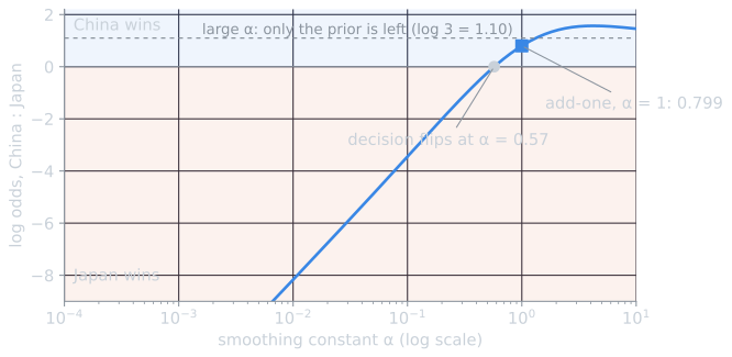
Near $\alpha = 0$ the log odds fall without limit, because $\hat{P}(\textit{Tokyo} \mid c)$ approaches zero. As $\alpha$ grows, the estimates for both classes approach the uniform $1/6$, the term evidence cancels, and only the prior's $\log 3 = 1.099$ remains. The decision changes from Japan to China at $\alpha = 0.573$. Smoothing is therefore not a technicality for avoiding zeros. It sets how far the classifier trusts sparse counts, and it should be chosen on held-out data, like any other parameter. The Reuters results below show what that looks like on a real collection.
Computing in log space
Multiplying hundreds of probabilities, each much smaller than 1, produces numbers too small to represent in floating point. A product of factors of $10^{-4}$, a typical probability for a moderately rare term, reaches zero in double precision after 81 factors, and the average Reuters story in the experiments below has 87.5 tokens after stop words are removed. Taking logarithms turns the product into a sum, and the logarithm preserves order:
$$c_{\text{map}} = \arg\max_{c} \left[ \log \hat{P}(c) + \sum_{k=1}^{n_d} \log \hat{P}(t_k \mid c) \right].$$
Each term adds evidence for or against each class, weighted by its log probability, and the prior is a starting bias toward common classes. For the running example, with natural logarithms:
| Contribution | China | Japan |
|---|---|---|
| Prior | log 3/4 = −0.288 | log 1/4 = −1.386 |
| Chinese (3 times) | 3 × (−0.847) = −2.542 | 3 × (−1.504) = −4.512 |
| Tokyo (once) | −2.639 | −1.504 |
| Japan (once) | −2.639 | −1.504 |
| Score | −8.108 | −8.907 |
China wins by 0.799. The table shows where the decision comes from. Japan gains 1.135 on each of Tokyo and Japan, 2.270 in all. China gains 0.657 on each of the three occurrences of Chinese, 1.970 in all, which by itself is not enough. It wins because the prior favours it by a further 1.099.
Naive Bayes is a linear classifier
For two classes, the decision depends only on the difference of the two scores, the log odds. Subtracting the two sums and grouping the tokens by term, so that a term occurring $\mathrm{tf}_{t,d}$ times contributes $\mathrm{tf}_{t,d}$ times:
$$\log \frac{\hat{P}(c \mid d)}{\hat{P}(\bar{c} \mid d)} = \underbrace{\log \frac{\hat{P}(c)}{\hat{P}(\bar{c})}}_{b} + \sum_{t \in V} \mathrm{tf}_{t,d} \underbrace{\log \frac{\hat{P}(t \mid c)}{\hat{P}(t \mid \bar{c})}}_{w_t}.$$
The document is assigned to $c$ when $b + \sum_t w_t \, \mathrm{tf}_{t,d} > 0$. That is a weighted sum of the document's term counts compared with a threshold, a hyperplane in the space of term-frequency vectors. Multinomial Naive Bayes is therefore a linear classifier, in the same family as the BIM's sum of term weights and the classifiers of vector space classification. Each weight $w_t$ is the log of how many times more probable the term is in one class than the other, and it can be read directly as that term's vote.
For the running example the weights are:
| Term | $w_t$ | Count in test document | Contribution |
|---|---|---|---|
| Chinese | log (6/14)/(2/9) = 0.657 | 3 | 1.970 |
| Beijing, Shanghai, Macao | log (2/14)/(1/9) = 0.251 | 0 | 0 |
| Tokyo | log (1/14)/(2/9) = −1.135 | 1 | −1.135 |
| Japan | log (1/14)/(2/9) = −1.135 | 1 | −1.135 |
| Bias $b$ | log 3 = 1.099 | 1.099 | |
| Log odds | 0.799 |
Terms absent from the document contribute nothing, whatever their weights. That is a property of the multinomial model, and the main point of contrast with the Bernoulli model, in which absences count.
On a real category the weights show what the classifier has learned. For the Reuters category grain, trained on all 7,769 training stories:
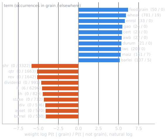
The positive weights are what a person would expect: feedgrain, wheat, maize, barley, durum, and rice. The largest weights go to terms that occur only in grain stories, such as feedgrain, 50 times in grain and never elsewhere. Smoothing caps them: a term never seen outside the class cannot receive an infinite weight, only one that grows with its count. The most negative weights belong to the vocabulary of earnings reports, the largest category in the collection. Most of the evidence that a story is not about grain is evidence that it is about something specific, such as quarterly results. The bias is $b = \log(433/7{,}336) = -2.830$, since only 433 of the 7,769 training stories are about grain. A story must collect about 2.8 nats of evidence before the classifier will assign it to the category.
Cost
Training reads every token once to count it, then computes a probability for every term in every class: $O(\lvert \mathbb{D} \rvert L_{\text{ave}} + \lvert \mathbb{C} \rvert \lvert V \rvert)$, where $L_{\text{ave}}$ is the average document length. Classifying a document adds one log probability per token per class: $O(\lvert \mathbb{C} \rvert L_d)$. Both are as cheap as a learning method can be, since even reading the data takes as long as training. That speed is a large part of why Naive Bayes is used on very large collections, such as the 120,000 reviews of my Goodreads project.
Results on Reuters-21578
The experiments in this topic use the ten largest categories of Reuters-21578 with its standard training and test split: 7,769 training stories and 3,019 test stories. A separate binary classifier was trained for each category, as is usual for multilabel collections. Text was lowercased, tokenized into alphabetic words, filtered with a short stop list (Lucene's English list plus said) and by removing one-letter tokens, and stemmed with the original Porter algorithm. With all 18,135 terms of the training vocabulary and add-one smoothing, multinomial Naive Bayes reached a micro-averaged F1 of 0.835 and a macro-averaged F1 of 0.721 on the test stories.
The per-category results show where it struggles:
| Category | F1 | Category | F1 |
|---|---|---|---|
| acq | 0.953 | interest | 0.706 |
| earn | 0.948 | money-fx | 0.703 |
| crude | 0.818 | wheat | 0.583 |
| ship | 0.765 | trade | 0.532 |
| grain | 0.710 | corn | 0.495 |
Large categories with distinctive vocabulary, such as earn and acq (acquisitions), are classified almost perfectly. Small categories that overlap with others, such as wheat and corn, nearly all of whose stories are also labeled grain, are much harder, because their stories share most of their vocabulary with stories about grain in general. The errors are lopsided: every category's recall is above 0.84, while precision falls as low as 0.35 for corn. The classifier assigns small categories too often. Evaluating classifiers gives the full counts and shows that moving the decision threshold above zero recovers much of the lost F1. Vector space classification compares other classifiers on the same data.
Choosing the smoothing constant
To see whether add-one is a good choice, the training stories were split at random (seed 790) into 80 percent for training and 20 percent for development, and $\alpha$ was varied:
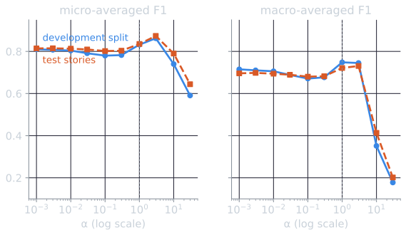
On the development split, $\alpha = 3$ gave the best micro-F1 (0.862) and $\alpha = 1$ the best macro-F1 (0.748), with $\alpha = 3$ close behind (0.745). Values of 10 and above collapsed, macro-F1 falling to 0.351 at $\alpha = 10$. A plausible reason is that heavy smoothing flattens the small categories' distributions toward uniform, which erases their distinctive terms, until the prior against a small category decides almost everything. Values below 1 were somewhat worse and nearly flat. The test results follow the development results closely, which is what a sound development split should show: with $\alpha = 3$, test micro-F1 rises from 0.835 to 0.874 and macro-F1 from 0.721 to 0.731. The best value depends on the collection, its vocabulary size, and the class sizes, so it should be tuned rather than assumed. The rest of this topic keeps $\alpha = 1$, so that its numbers stay comparable.
References
- Lewis, D. D. (1998). Naive (Bayes) at forty: The independence assumption in information retrieval. In Proceedings of ECML 1998, 4–15.
- Manning, C. D., Raghavan, P., and Schütze, H. (2008). Introduction to Information Retrieval, sections 13.2 and 13.4. Cambridge University Press.