K-means is the most widely used clustering algorithm, in text processing and well beyond it. It represents each cluster by a single point, its centroid, and alternates between two simple steps: assign every document to its nearest centroid, then move every centroid to the mean of its documents. The procedure is easy to state, fast enough for large collections, and guaranteed to stop. What it finds when it stops, and how much that depends on where it started, are the questions that K-means in practice takes up. This article covers the algorithm itself, following Manning, Raghavan, and Schütze (2008, §16.4), and traces it by hand on six points so that every number can be checked.
The objective
Documents are represented as vectors, usually length-normalized TF-IDF vectors, so that the Euclidean distance between two documents reflects their cosine similarity. The goal is to divide $N$ document vectors $\vec{x}_1, \dots, \vec{x}_N$ into $K$ clusters $\omega_1, \dots, \omega_K$, where $K$ is chosen in advance. Each cluster has a centroid, the mean of its members:
$$\vec{\mu}(\omega_k) = \frac{1}{\lvert \omega_k \rvert} \sum_{\vec{x} \in \omega_k} \vec{x}.$$
A good clustering has members close to their centroids. K-means measures this with the residual sum of squares (RSS), the total squared distance from each document to its cluster's centroid:
$$\mathrm{RSS} = \sum_{k=1}^{K} \sum_{\vec{x} \in \omega_k} \lvert \vec{x} - \vec{\mu}(\omega_k) \rvert^2.$$
Each inner sum is the RSS of one cluster, written $\mathrm{RSS}_k$. Smaller RSS means tighter clusters, and K-means tries to minimize it. The distances are squared, which has two consequences used below: the best single point to represent a cluster is exactly its mean, and a document far from its centroid costs far more than one near it, so outliers pull hard on the result.
Finding the clustering with the smallest possible RSS is computationally hard. It is NP-hard even for two clusters in general dimensions (Aloise, Deshpande, Hansen, and Popat, 2009), and the number of candidate clusterings grows explosively: six points can be split into two nonempty clusters in $2^5 - 1 = 31$ ways, and a few thousand documents into six clusters in more ways than there are atoms in the universe. K-means settles for a heuristic that improves the clustering step by step.
The algorithm
The algorithm is usually credited to Stuart Lloyd, who described it in 1957 in a report published only in 1982 (Lloyd, 1982), and to James MacQueen, who gave it the name K-means (MacQueen, 1967).
- Initialize. Choose $K$ starting centroids, for example $K$ documents picked at random. These are called the seeds.
- Assign. Assign each document to the cluster whose centroid is nearest.
- Update. Recompute each centroid as the mean of the documents now assigned to it.
- Repeat steps 2 and 3 until the assignments stop changing, or another stopping criterion is met: a fixed number of iterations, centroids that no longer move, or RSS that falls by less than a threshold.
The two steps solve two easier halves of the hard problem. With the centroids held fixed, the best assignment is obvious: send each document to its nearest centroid. With the assignment held fixed, the best centroids are obvious too: the means. K-means alternates between the two halves, each time solving one exactly while holding the other fixed.
A worked example
Six points in two dimensions, clustered into $K = 2$ clusters, with points $A$ and $B$ as the seeds:
| Point | A | B | C | D | E | F |
|---|---|---|---|---|---|---|
| Coordinates | (1, 1) | (1.5, 2) | (3, 4) | (5, 7) | (3.5, 5) | (4.5, 5) |
The table below gives, for each point and each iteration, the squared distance to the first centroid, then to the second, and the cluster the point is assigned to. Squared distances are enough for the assignment, since the nearer centroid is the same whether distances are squared or not, and they are what RSS adds up. All values are exact.
| Point | Iteration 1: centroids (1, 1), (1.5, 2) | Iteration 2: centroids (1, 1), (3.5, 4.6) | Iteration 3: centroids (1.25, 1.5), (4, 5.25) |
|---|---|---|---|
| A | 0 / 1.25 → 1 | 0 / 19.21 → 1 | 0.3125 / 27.0625 → 1 |
| B | 1.25 / 0 → 2 | 1.25 / 10.76 → 1 | 0.3125 / 16.8125 → 1 |
| C | 13 / 6.25 → 2 | 13 / 0.61 → 2 | 9.3125 / 2.5625 → 2 |
| D | 52 / 37.25 → 2 | 52 / 8.01 → 2 | 44.3125 / 4.0625 → 2 |
| E | 22.25 / 13 → 2 | 22.25 / 0.16 → 2 | 17.3125 / 0.3125 → 2 |
| F | 28.25 / 18 → 2 | 28.25 / 1.16 → 2 | 22.8125 / 0.3125 → 2 |
Iteration 1. With centroids at $A = (1, 1)$ and $B = (1.5, 2)$, point $A$ is nearest the first centroid, and every other point, including $B$ itself, is nearest the second. The clusters are $\{A\}$ and $\{B, C, D, E, F\}$. RSS, measured from the seeds, is the sum of each point's distance to its own centroid: $0 + 0 + 6.25 + 37.25 + 13 + 18 = 74.5$. Updating leaves the first centroid at $A$ and moves the second to the mean of its five points,
$$\left(\tfrac{1.5 + 3 + 5 + 3.5 + 4.5}{5},\ \tfrac{2 + 4 + 7 + 5 + 5}{5}\right) = (3.5,\ 4.6),$$
and RSS falls to 20.7.
Iteration 2. Point $B$ is now at squared distance 1.25 from $(1, 1)$ and 10.76 from $(3.5, 4.6)$, so it changes cluster. That single move lowers RSS by $10.76 - 1.25 = 9.51$, from 20.7 to 11.19. The clusters are $\{A, B\}$ and $\{C, D, E, F\}$. Updating moves the centroids to $(1.25, 1.5)$ and $(4, 5.25)$, and RSS falls to 7.875.
Iteration 3. No point changes cluster, so the centroids do not move, and the algorithm stops with RSS 7.875.
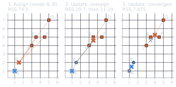
| Step | Clusters | RSS |
|---|---|---|
| Assignment 1 | {A}, {B, C, D, E, F} | 74.5 |
| Update 1 | same | 20.7 |
| Assignment 2 | {A, B}, {C, D, E, F} | 11.19 |
| Update 2 | same | 7.875 |
| Assignment 3 | no change: stop | 7.875 |
RSS fell at every step. That is not a coincidence, and the next section shows why. This clustering is also the best possible one: checking all 31 ways of splitting the six points in two, none has RSS below 7.875. The next best, $\{A, B, C\}$ and $\{D, E, F\}$, has 10.67, and it will reappear below.
Why K-means converges
The argument has three parts: the assignment step never increases RSS, the update step never increases RSS, and RSS cannot decrease forever (Manning, Raghavan, and Schütze, 2008, §16.4).
The assignment step
RSS is a sum of one term per document, its squared distance to the centroid of the cluster it belongs to. With the centroids fixed, each term depends only on that document's own assignment, so the sum is smallest when each document is assigned to minimize its own term, which is exactly what the assignment step does. A document that moves goes from a centroid at squared distance $d_{\text{old}}$ to one at $d_{\text{new}} < d_{\text{old}}$, and RSS drops by $d_{\text{old}} - d_{\text{new}}$. Iteration 2 above shows this with $B$: $10.76 - 1.25 = 9.51$.
The update step
With the assignment fixed, the clusters can be treated one at a time, since moving one cluster's centroid changes only that cluster's term. For cluster $\omega_k$ with $n_k$ members, consider its RSS as a function of where the centroid is put, a free point $\vec{v}$ with components $v_1, \dots, v_M$:
$$\mathrm{RSS}_k(\vec{v}) = \sum_{\vec{x} \in \omega_k} \lvert \vec{v} - \vec{x} \rvert^2 = \sum_{\vec{x} \in \omega_k} \sum_{m=1}^{M} (v_m - x_m)^2.$$
This is a sum of squares in each coordinate separately, so it can be minimized one coordinate at a time. Its partial derivative in $v_m$ is
$$\frac{\partial\, \mathrm{RSS}_k(\vec{v})}{\partial v_m} = \sum_{\vec{x} \in \omega_k} 2 (v_m - x_m) = 2 n_k v_m - 2 \sum_{\vec{x} \in \omega_k} x_m.$$
Setting it to zero gives $v_m = \frac{1}{n_k} \sum_{\vec{x} \in \omega_k} x_m$, the $m$th coordinate of the mean. The second derivative is $2 n_k > 0$, so this is a minimum, not a maximum. The mean is therefore the unique best position for the centroid, and replacing the old centroid with the mean can only lower $\mathrm{RSS}_k$ (Manning, Raghavan, and Schütze, 2008, §16.4).
A second way to see the same fact also says how much RSS falls. Write $\vec{\mu}$ for the mean of the cluster and expand each squared distance around it:
$$\lvert \vec{x} - \vec{v} \rvert^2 = \lvert (\vec{x} - \vec{\mu}) + (\vec{\mu} - \vec{v}) \rvert^2 = \lvert \vec{x} - \vec{\mu} \rvert^2 + 2 (\vec{x} - \vec{\mu}) \cdot (\vec{\mu} - \vec{v}) + \lvert \vec{\mu} - \vec{v} \rvert^2.$$
Summing over the cluster, the middle term vanishes, because $\sum_{\vec{x}} (\vec{x} - \vec{\mu}) = n_k \vec{\mu} - n_k \vec{\mu} = \vec{0}$. What remains is
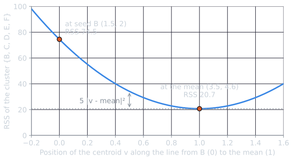
$$\mathrm{RSS}_k(\vec{v}) = \mathrm{RSS}_k(\vec{\mu}) + n_k \lvert \vec{\mu} - \vec{v} \rvert^2.$$
Moving a centroid from $\vec{v}$ to the mean lowers RSS by exactly $n_k$ times the squared distance it moves. In the example's first update, the second centroid moved from $(1.5, 2)$ to $(3.5, 4.6)$, a squared distance of $2^2 + 2.6^2 = 10.76$, with five members, so RSS fell by $5 \times 10.76 = 53.8$, from 74.5 to 20.7. In the second update, the centroids moved by squared distances $0.3125$ and $0.6725$ with two and four members, lowering RSS by $0.625 + 2.69 = 3.315$, from 11.19 to 7.875.
Termination
RSS therefore never increases. There are finitely many ways to assign $N$ documents to $K$ clusters, and each set of assignments determines its centroids and so its RSS. As long as the algorithm changes the assignment only when RSS strictly falls, it can never return to a clustering it has left, so it must reach, after finitely many steps, a clustering where neither step changes anything. The finite count gives no useful bound on the number of iterations, but in most cases the algorithm quickly reaches convergence, or a clustering close enough to it that further iterations would move only a few documents (Manning, Raghavan, and Schütze, 2008, §16.4).
The proviso about strict decrease is why ties need care. A document equally close to two centroids contributes the same to RSS in either cluster, and if ties were broken differently from one iteration to the next, the algorithm could cycle among clusterings of equal cost. The fix is a consistent rule: a document equally close to two centroids stays where it is, or goes to the cluster with the lower index (Manning, Raghavan, and Schütze, 2008, §16.4).
Local minima
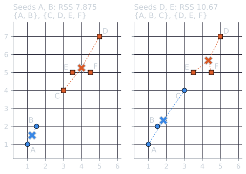
Convergence is guaranteed, but only to a local minimum: a clustering that neither step can improve, which may still be far from the best possible. The same six points show it. Start from seeds $D = (5, 7)$ and $E = (3.5, 5)$ instead of $A$ and $B$. Every point except $D$ is nearer $E$, so the first clusters are $\{D\}$ and $\{A, B, C, E, F\}$. The second centroid moves to $(2.7, 3.4)$, which leaves $F$ nearer $D$, so $F$ switches in the second iteration; the centroids move again, and $E$ follows in the third. In the fourth iteration nothing changes, and the algorithm stops at $\{A, B, C\}$ and $\{D, E, F\}$, with centroids $(1.83, 2.33)$ and $(4.33, 5.67)$ (rounded). RSS fell through 37.5, 21.5, 19.95, 16.375 and 13.375 to 10.67, decreasing at every step exactly as the proof requires, and still ended higher than before.
Neither step can improve this clustering. The only point near the boundary is $C$, at squared distance $1.17^2 + 1.67^2 \approx 4.14$ from the first centroid and $1.33^2 + 1.67^2 \approx 4.56$ from the second, so it stays; the centroids are already the means; and so the algorithm stops, at an RSS 35 percent above the optimum of 7.875. Of the 15 possible pairs of seeds, 7 lead to the optimum and 8 to this local minimum.
How much worse can a local minimum be? Without limit. Take four points at the corners of a rectangle 6 wide and 2 high, $(0, 0)$, $(0, 2)$, $(6, 0)$ and $(6, 2)$, with $K = 2$. The natural clustering pairs the two left corners and the two right corners, with RSS $4 \times 1^2 = 4$. If both seeds are left corners, the first assignment pairs each left corner with the right corner at the same height, giving top and bottom clusters with centroids $(3, 0)$ and $(3, 2)$. Every point is 3 from its own centroid and $\sqrt{13} \approx 3.6$ from the other, so nothing moves, and K-means stops with RSS $4 \times 3^2 = 36$, nine times the optimum. Stretching the rectangle makes the ratio as large as desired.
The result depends on the starting centroids, and starting from points that lie in the same natural group can split that group in two and merge two others. The standard remedies are to run K-means several times from different starting points and keep the clustering with the lowest RSS, and to choose starting points more carefully. K-means in practice works out how much careful seeding (k-means++) helps on these two examples and measures both remedies on Reuters news stories.
Stepping through K-means
The demo runs the algorithm one half-iteration at a time on the six points above, on the rectangle, or on three blobs of points. The shaded regions show which centroid is nearest each part of the plane, so they are the regions the next assignment step will use. Dragging a point, or clicking an empty spot to add one, restarts the run from the same seeds. With seeds A and B, the readout repeats the RSS sequence of the worked example; with seeds D and E it ends at 10.67.
Cost
Each iteration computes the distance from each of $N$ documents to each of $K$ centroids, in a space of $M$ dimensions, so the assignment step costs $O(KNM)$. The update step adds each document to one centroid, $O(NM)$. With $I$ iterations the total is $O(IKNM)$, linear in the number of documents, which is what makes K-means practical for large collections (Manning, Raghavan, and Schütze, 2008, §16.4). For scale: the Reuters experiment in K-means in practice has $N = 7{,}487$ stories, $M = 3{,}000$ terms and $K = 6$, so one assignment step is about 135 million multiply-adds, a fraction of a second on a laptop.
Text adds a wrinkle. Document vectors are sparse, but centroids, averages of many documents, are dense, since they contain every term that appears in any member. Distance computations with dense centroids lose the advantage of sparsity. Implementations often keep only each centroid's highest-weighted terms, or use the dot product between a sparse document and a dense centroid, which costs time proportional to the number of terms in the document rather than the vocabulary. The dot product is enough because, for a unit-length document $\vec{x}$, $\lvert \vec{x} - \vec{\mu} \rvert^2 = 1 - 2\, \vec{x} \cdot \vec{\mu} + \lvert \vec{\mu} \rvert^2$, and $\lvert \vec{\mu} \rvert^2$ is computed once per centroid per iteration.
Related algorithms
K-means is a special case of a more general method. The expectation-maximization (EM) algorithm fits a mixture of probability distributions. The 2-Poisson model of term frequency can be fitted this way, as it was in that article. With Gaussian clusters of equal, fixed variance, as the variance shrinks, EM becomes K-means: the soft assignment of each document to clusters by probability becomes the hard assignment to the nearest centroid. EM with a full mixture model gives a soft clustering, assigning each document a degree of membership in every cluster (Manning, Raghavan, and Schütze, 2008, §16.5).
The worked example and both local-minimum examples are recomputed by tools/experiments/clustering/lloyd_worked.py in the site repository.
References
- Aloise, D., Deshpande, A., Hansen, P., and Popat, P. (2009). NP-hardness of Euclidean sum-of-squares clustering. Machine Learning, 75(2), 245–248.
- Lloyd, S. P. (1982). Least squares quantization in PCM. IEEE Transactions on Information Theory, 28(2), 129–137.
- MacQueen, J. (1967). Some methods for classification and analysis of multivariate observations. In Proceedings of the Fifth Berkeley Symposium on Mathematical Statistics and Probability, 281–297.
- Manning, C. D., Raghavan, P., and Schütze, H. (2008). Introduction to Information Retrieval, sections 16.4–16.5. Cambridge University Press.