In the Cranfield collection of 1,400 aerodynamics abstracts, the word flutter appears in 56 documents. If occurrences of a word were scattered at random through the text, like typing errors, its count per document would follow a Poisson distribution, and with the collection's average of 0.2 occurrences per document, essentially no document would contain it six or more times. In fact 22 documents do. The counts do not look random at all. Most documents never mention flutter. A small group mention it again and again, because they are about flutter.
That observation is the basis of the 2-Poisson model, which describes a term's frequency in a document as depending on whether the document is about the term's concept. The model is too complex to use directly in ranking, but its shape is the source of the term frequency saturation in BM25. This article explains the model, fits it to real term counts, computes the term weight it implies from Cranfield's relevance judgments, and follows the path from that weight to the BM25 formula. The fits come from tools/experiments/cranfield/twopois.py and twopois_eliteness.py (terms are stemmed, so boundary appears in the data as boundari).
Why a single Poisson fails
The Poisson distribution describes counts of events that occur independently at a constant average rate. With mean $\lambda$, the probability of exactly $k$ occurrences is
$$P(k) = \frac{e^{-\lambda} \lambda^k}{k!}.$$
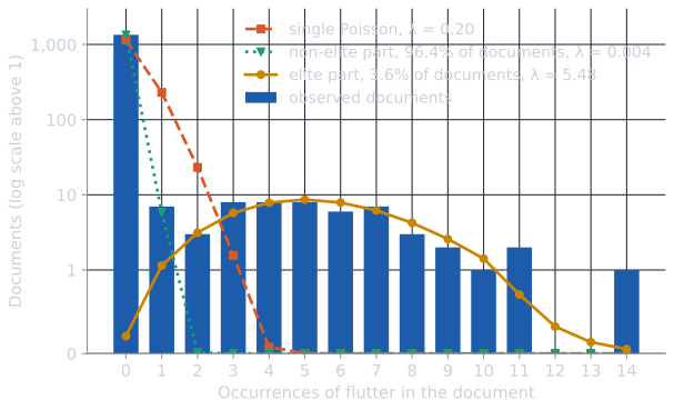
If a term occurred at a constant rate throughout the collection, its count in a document would be Poisson with $\lambda$ equal to its average count per document. Fitting that model to four Cranfield terms, after stemming, and comparing its predictions with the actual number of documents at each count shows how badly it fails. For flutter:
| Occurrences in document | 0 | 1 | 2 | 3 | 4 | 5 | 6 or more |
|---|---|---|---|---|---|---|---|
| Documents observed | 1,344 | 7 | 3 | 8 | 8 | 8 | 22 |
| Single Poisson, $\lambda = 0.20$ | 1,144.6 | 230.6 | 23.2 | 1.6 | 0.1 | 0.0 | 0.0 |
The single Poisson predicts far too few documents with no occurrences, far too many with exactly one, and almost none with many. The real distribution has two humps: a large mass at zero and a long tail of documents that use the word heavily. The same pattern holds for every content-bearing term examined. Function words such as the behave much more like a single Poisson, since every document uses them at roughly the rate its length dictates.
The 2-Poisson mixture
Bookstein and Swanson (1974) and Harter (1975) proposed that a content term divides the documents into two classes:
- Elite documents are about the concept the term represents. In them the term occurs at a high rate, $\lambda_E$.
- Non-elite documents are not about the concept. In them the term occurs only incidentally, at a low rate, $\lambda_N$.
If a fraction $\pi$ of documents is elite, the count of the term in a random document follows a mixture of two Poisson distributions:
$$P(k) = \pi\, \frac{e^{-\lambda_E} \lambda_E^k}{k!} + (1 - \pi)\, \frac{e^{-\lambda_N} \lambda_N^k}{k!}.$$
The model can be read as a story of how a document is written (Robertson and Zaragoza, 2009, §3.4.1). The author first decides, for each term, whether the document will be about that term's concept. Then the words are written, and each word position is filled with the term at the rate its class dictates. The decision is invisible; only the counts are observed.
Fitting the mixture by EM
The three parameters can be estimated from the observed counts with the expectation-maximization (EM) algorithm. If we knew which documents were elite, estimating the parameters would be easy: $\pi$ would be the elite fraction and each $\lambda$ the average count in its class. If we knew the parameters, computing each document's probability of being elite would be easy too, by Bayes' rule. EM alternates between the two.
- Start from a guess. The experiment starts at $\pi = 0.1$, $\lambda_E = \max(5\bar{k}, 1)$, and $\lambda_N = 0.3\bar{k} + 0.001$, where $\bar{k}$ is the mean count.
- E-step. For each document $d$ with count $k_d$, compute its posterior probability of being elite: $$r_d = \frac{\pi\, \mathrm{Pois}(k_d; \lambda_E)}{\pi\, \mathrm{Pois}(k_d; \lambda_E) + (1 - \pi)\, \mathrm{Pois}(k_d; \lambda_N)}.$$
- M-step. Re-estimate the parameters as if each document were elite with weight $r_d$: $$\pi = \frac{1}{n} \sum_d r_d, \qquad \lambda_E = \frac{\sum_d r_d\, k_d}{\sum_d r_d}, \qquad \lambda_N = \frac{\sum_d (1 - r_d)\, k_d}{\sum_d (1 - r_d)}.$$
- Repeat steps 2 and 3. Each round cannot decrease the likelihood of the data.
For flutter, the first rounds run as follows (log-likelihood in natural logs):
| Iteration | $\pi$ | $\lambda_E$ | $\lambda_N$ | Log-likelihood |
|---|---|---|---|---|
| 0 (start) | 0.1000 | 1.007 | 0.0614 | −656.26 |
| 1 | 0.0766 | 2.586 | 0.0036 | −434.93 |
| 2 | 0.0451 | 4.450 | 0.0010 | −374.00 |
| 3 | 0.0391 | 5.113 | 0.0015 | −369.53 |
| 4 | 0.0375 | 5.294 | 0.0028 | −368.08 |
| 6 | 0.0361 | 5.463 | 0.0042 | −367.61 |
| 10 and after | 0.0360 | 5.485 | 0.0044 | −367.60 |
The first E-step sees that documents with many occurrences are far better explained by the high-rate class, so the elite rate jumps, and the elite class shrinks to the documents that really use the word. By iteration 10 the estimates no longer change at four decimals. Fitted to the Cranfield counts:
| Term | Documents containing it | Elite fraction $\pi$ | $\lambda_E$ | $\lambda_N$ |
|---|---|---|---|---|
| flutter | 56 | 0.036 | 5.48 | 0.004 |
| shock | 240 | 0.121 | 4.41 | 0.063 |
| heat | 306 | 0.170 | 3.81 | 0.065 |
| boundary | 469 | 0.240 | 3.71 | 0.144 |
The mixture's predictions for flutter are 1,344.0, 7.0, 3.2, 5.7, 7.9, 8.6, and 23.6 documents at counts 0 through 6 or more. They are nearly identical to the observed 1,344, 7, 3, 8, 8, 8, and 22. About 3.6 percent of the documents, roughly 50, are elite for flutter and mention it about five and a half times on average. The rest almost never mention it. For the other three terms, the mixture is far closer than a single Poisson but not exact. For shock it predicts 22 documents with two occurrences where there are 38, and for boundary it misses the counts at three and four occurrences by about a dozen documents each. Two classes capture most of the structure, not all of it. Boundary, a very common concept in aerodynamics, has nearly a quarter of the collection in its elite set.
Eliteness and relevance
The model's central idea is eliteness: a hidden property of a document-term pair, whether the document is about the term's concept. Term frequency is evidence of eliteness, and eliteness, not frequency itself, is what relates to relevance. A document relevant to a query about flutter is likely to be elite for flutter. Seeing the word many times makes eliteness more probable, but only up to a point. Once a document is clearly elite, further occurrences say little more.
How fast the evidence accumulates
The E-step's posterior $r_d$ is exactly the probability that a document is elite given its count, and it can be tabulated. For flutter and one occurrence, the elite class explains the count with probability $0.036 \times e^{-5.485} \times 5.485 = 0.00082$ and the non-elite class with $0.964 \times e^{-0.00436} \times 0.00436 = 0.00418$ (the fitted $\lambda_N$ is 0.00436 before rounding), so
$$P(\text{elite} \mid \mathit{tf} = 1) = \frac{0.00082}{0.00082 + 0.00418} = 0.164.$$
A single mention is more likely incidental than topical. At two occurrences the non-elite class, with its rate of 0.0044, can hardly produce the count at all, and the posterior jumps to 0.996.
| Term | tf = 0 | tf = 1 | tf = 2 | tf = 3 | tf = 4 |
|---|---|---|---|---|---|
| flutter | 0.000 | 0.164 | 0.996 | 1.000 | 1.000 |
| shock | 0.002 | 0.111 | 0.898 | 0.998 | 1.000 |
| heat | 0.005 | 0.222 | 0.944 | 0.999 | 1.000 |
| boundary | 0.009 | 0.187 | 0.856 | 0.994 | 1.000 |
For all four terms, the second and third occurrences settle the question. A document with 20 occurrences is no more elite than one with 4. This is the saturation that BM25 builds in.
The eliteness term weight
Robertson, van Rijsbergen, and Porter (1981) built a retrieval model on this idea, in which eliteness, not the term itself, is what relevance depends on. Write $p_1 = P(\text{elite} \mid R = 1)$ and $p_0 = P(\text{elite} \mid R = 0)$ for how often relevant and nonrelevant documents are elite for the term, and $E_1(\mathit{tf})$ and $E_0(\mathit{tf})$ for the elite and non-elite Poisson probabilities of a count. The probability of a count in a relevant document is $p_1 E_1(\mathit{tf}) + (1 - p_1) E_0(\mathit{tf})$, and similarly with $p_0$ for a nonrelevant one. Taking the log odds ratio of a count $\mathit{tf}$ against a count of zero, exactly as the BIM takes the log odds ratio of presence against absence, gives the term weight (Robertson and Zaragoza, 2009, eq. 3.6):
$$w(\mathit{tf}) = \log \frac{\big(p_1 E_1(\mathit{tf}) + (1 - p_1) E_0(\mathit{tf})\big)\,\big(p_0 E_1(0) + (1 - p_0) E_0(0)\big)}{\big(p_1 E_1(0) + (1 - p_1) E_0(0)\big)\,\big(p_0 E_1(\mathit{tf}) + (1 - p_0) E_0(\mathit{tf})\big)}.$$
The weight is zero at $\mathit{tf} = 0$ by construction. As $\mathit{tf}$ grows, the elite distribution dominates both mixtures, and the weight approaches the weight that eliteness itself would have if it could be observed, the BIM weight of the eliteness feature, $\log \frac{p_1 (1 - p_0)}{(1 - p_1) p_0}$ (their eq. 3.8). That limit drops two small terms, $p_1 E_1(0)$ and $p_0 E_1(0)$, the chance that an elite document contains no occurrence at all. Keeping them gives a slightly lower exact limit.
Cranfield's relevance judgments allow every quantity in this weight to be estimated. The Poisson rates come from the EM fit above. For $p_1$ and $p_0$, take the Cranfield queries that contain the term and average the posterior eliteness of their judged relevant documents and of all their other documents. For flutter, 11 queries contain the word, with 75 (query, relevant document) pairs between them:
| Term | Queries | $p_1$ | $p_0$ | $w(1)$ | $w(2)$ | $w(3)$ | Limit, eq. 3.8 | Exact limit |
|---|---|---|---|---|---|---|---|---|
| flutter | 11 | 0.791 | 0.032 | 2.86 | 4.71 | 4.72 | 4.73 | 4.72 |
| shock | 10 | 0.657 | 0.117 | 0.87 | 2.54 | 2.64 | 2.67 | 2.65 |
| heat | 23 | 0.653 | 0.167 | 1.00 | 2.14 | 2.20 | 2.23 | 2.20 |
| boundary | 28 | 0.728 | 0.237 | 0.81 | 1.95 | 2.08 | 2.15 | 2.09 |
Relevant documents are elite for the query's terms most of the time (65 to 79 percent), and nonrelevant ones rarely. The weight rises from zero, reaches 93 to nearly 100 percent of its limit by the second occurrence, and is flat from the third. One more feature is visible: for shock, heat, and boundary, the second occurrence adds more weight than the first. A single mention is weak evidence of eliteness, the second is strong, and the weight follows the posterior. Robertson and Zaragoza (2009, §3.4.4) describe this initial upturn as possible for some parameter combinations, with most combinations giving a curve that bends down from the start.
But the full model needed four parameters per term, none of them directly observable because eliteness is hidden. Estimating them here took relevance judgments for many queries and an EM fit per term, and in experiments the model gained little over simpler weights.
From the model to BM25
Robertson and Walker (1994) took a different approach. Instead of estimating the 2-Poisson model, they designed a simple function with the same qualitative shape:
$$\frac{\mathit{tf}}{\mathit{tf} + k_1}.$$
It is 0 at $\mathit{tf} = 0$, increases with every occurrence, and approaches 1 as $\mathit{tf}$ grows. The single parameter $k_1$ controls how quickly it saturates. They multiplied it by the Robertson–Spärck Jones weight of the Binary Independence Model, which stands in for the model's asymptotic maximum. They then added document length normalization, motivated by the same model. If a document is long because it is verbose, both of its Poisson rates are higher in proportion to its length, so its counts should be scaled down to be comparable with a shorter document's. The result, after experiments at TREC, was BM25 (see Okapi BM25), which also scales the saturation function by $k_1 + 1$ so that a single occurrence in a document of average length keeps the binary model's weight. Robertson and Zaragoza (2009) describe this step as fitting a simple curve to the shape of the model's weight function rather than estimating the model itself. The approach keeps the behavior that the theory predicts while avoiding parameters that cannot be estimated.
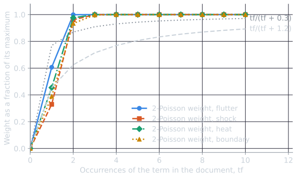
The comparison in the figure is informative in both directions. The shape is right: zero at zero, rising, leveling off. The speed differs: the fitted 2-Poisson weight is essentially flat after three occurrences, while $\mathit{tf}/(\mathit{tf} + 1.2)$ is still at 71 percent of its limit at $\mathit{tf} = 3$ and 89 percent at $\mathit{tf} = 10$. Two features of real text that the model leaves out plausibly account for some of the gap. The model treats every document as the same length, so a long abstract that is elite for flutter and a short one are expected to use the word equally often. And it allows only two levels of aboutness, so a document entirely devoted to flutter and one with a paragraph on it are both just "elite". Real collections, where repetition carries some further evidence of how central a topic is, are better served by a gentler curve, and on Cranfield the tuned $k_1$ in comparing ranking models is 1.5, not 0.3.
The data in this article show why saturation is right. For a term like flutter, a document with 2 occurrences is very probably elite, and one with 20 is no more elite than one with 6. Linear term frequency, as in raw TF-IDF, keeps rewarding repetition long after eliteness is settled. The saturating curve stops.
Limits
The 2-Poisson model is itself a simplification. It ignores document length, although longer documents naturally contain more occurrences. It assumes exactly two classes, though some terms seem to have degrees of aboutness. And it treats each term separately, ignoring that elite sets for related terms overlap. Its lasting value is not as a model to estimate but as an explanation of why term frequency matters and why its effect should diminish.
References
- Bookstein, A., and Swanson, D. R. (1974). Probabilistic models for automatic indexing. Journal of the American Society for Information Science, 25(5), 312–316.
- Harter, S. P. (1975). A probabilistic approach to automatic keyword indexing. Part I: On the distribution of specialty words in a technical literature. Journal of the American Society for Information Science, 26(4), 197–206.
- Robertson, S. E., van Rijsbergen, C. J., and Porter, M. F. (1981). Probabilistic models of indexing and searching. In R. N. Oddy et al. (Eds.), Information Retrieval Research, 35–56. Butterworths.
- Robertson, S. E., and Walker, S. (1994). Some simple effective approximations to the 2-Poisson model for probabilistic weighted retrieval. In Proceedings of SIGIR 1994, 232–241.
- Robertson, S., and Zaragoza, H. (2009). The probabilistic relevance framework: BM25 and beyond. Foundations and Trends in Information Retrieval, 3(4), 333–389.