A ranked system does not return a set. It returns an ordered list, and a user reads it from the top until satisfied or discouraged. Two rankings can contain the same documents and be very different in quality: one puts the relevant documents first, the other buries them at the bottom. Measures for rankings must therefore reward relevant documents for appearing early. All of them start from the same computation: precision and recall for the top $k$ results, for each $k$.
This article works through one ranking and computes the standard measures for it, following Manning, Raghavan, and Schütze (2008, §8.4). Mean average precision and nDCG, the two most widely reported measures, have their own articles and continue the same example. The numbers are computed by tools/experiments/eval_measures/worked_examples.py and cranfield_measures.py in the site's repository and rounded to three decimals.
A worked ranking
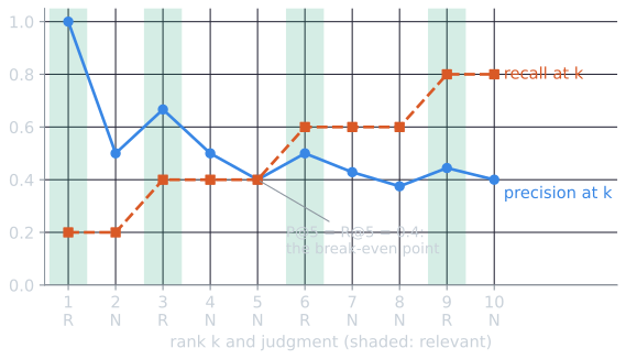
A query has 5 relevant documents in the collection. A system returns 10 documents, of which these ranks are relevant (R) or not (N):
| Rank $k$ | Judgment | Relevant so far | Precision at $k$ | Recall at $k$ |
|---|---|---|---|---|
| 1 | R | 1 | 1.000 | 0.2 |
| 2 | N | 1 | 0.500 | 0.2 |
| 3 | R | 2 | 0.667 | 0.4 |
| 4 | N | 2 | 0.500 | 0.4 |
| 5 | N | 2 | 0.400 | 0.4 |
| 6 | R | 3 | 0.500 | 0.6 |
| 7 | N | 3 | 0.429 | 0.6 |
| 8 | N | 3 | 0.375 | 0.6 |
| 9 | R | 4 | 0.444 | 0.8 |
| 10 | N | 4 | 0.400 | 0.8 |
Precision at $k$ is the number of relevant documents in the top $k$ divided by $k$. Recall at $k$ is that number divided by 5, the total number of relevant documents. The fifth relevant document is never retrieved, so recall never reaches 1.
The two columns behave differently as $k$ grows. Recall is a staircase: it moves up by $1/5$ at each relevant document and is flat otherwise, so it can never fall. Precision moves at every rank. At a relevant document it rises, because the numerator and denominator both grow by one and $(h+1)/(k+1) \ge h/k$ whenever $h \le k$. At a nonrelevant document it falls from $h/k$ to $h/(k+1)$.
The precision-recall curve
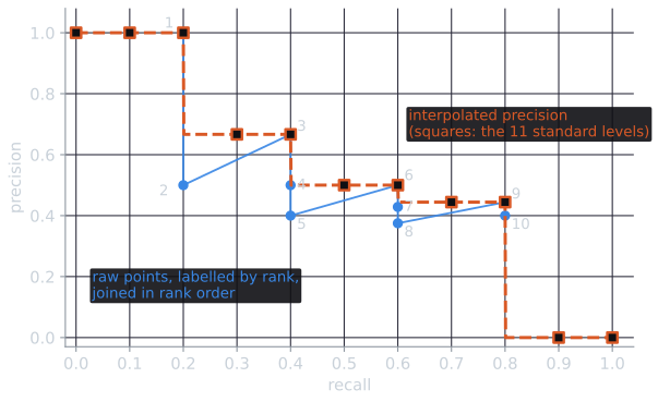
Plotting precision against recall, one point per rank, gives a precision-recall curve. Its characteristic shape is a sawtooth. Each relevant document raises recall and does not lower precision, a step to the right and usually up. Each nonrelevant document leaves recall unchanged and lowers precision, a drop straight down. In the table, precision rises to 0.667 at rank 3, falls to 0.4 by rank 5, rises to 0.5 at rank 6, and so on. Several ranks share a recall value: ranks 3, 4 and 5 all sit at recall 0.4, stacked vertically at precision 0.667, 0.5 and 0.4.
Interpolation
The sawtooth makes curves hard to compare and average. The standard fix is interpolated precision: the interpolated precision at recall level $r$ is the highest precision at any recall level $r' \ge r$,
$$p_{\text{interp}}(r) = \max_{r' \ge r} p(r').$$
The justification is that a user willing to read further to reach a higher recall would accept that extra effort if precision were at least as good, so the best precision achievable at or beyond a recall level is the meaningful one. Interpolation turns the sawtooth into a curve that never increases as recall grows.
Because recall only grows with rank, "recall at least $r$" means "rank at least the first rank where recall reaches $r$". So the interpolated precision at each point is a running maximum of precision taken from the bottom of the ranking upward. Working from rank 10 back to rank 1:
| Rank $k$ | Precision at $k$ | Recall at $k$ | Max precision at rank $k$ or below |
|---|---|---|---|
| 10 | 0.400 | 0.8 | 0.400 |
| 9 | 0.444 | 0.8 | 0.444 |
| 8 | 0.375 | 0.6 | 0.444 |
| 7 | 0.429 | 0.6 | 0.444 |
| 6 | 0.500 | 0.6 | 0.500 |
| 5 | 0.400 | 0.4 | 0.500 |
| 4 | 0.500 | 0.4 | 0.500 |
| 3 | 0.667 | 0.4 | 0.667 |
| 2 | 0.500 | 0.2 | 0.667 |
| 1 | 1.000 | 0.2 | 1.000 |
Reading off the last column at the first rank of each recall value gives the interpolated curve: 1.000 for recall up to 0.2 (rank 1), 0.667 up to 0.4 (rank 3), 0.500 up to 0.6 (rank 6), 0.444 up to 0.8 (rank 9), and 0 beyond 0.8, which the system never reaches.
The 11-point average
A traditional summary measures interpolated precision at the eleven recall levels 0.0, 0.1, ..., 1.0. For the example:
| Recall level | 0.0 | 0.1 | 0.2 | 0.3 | 0.4 | 0.5 | 0.6 | 0.7 | 0.8 | 0.9 | 1.0 |
|---|---|---|---|---|---|---|---|---|---|---|---|
| Interpolated precision | 1.000 | 1.000 | 1.000 | 0.667 | 0.667 | 0.500 | 0.500 | 0.444 | 0.444 | 0 | 0 |
At recall 0.3, the best precision at any recall of 0.3 or more is 0.667, reached at rank 3 with recall 0.4. At recall 0.9 and 1.0 the interpolated precision is 0, because the system never reaches those recall levels. The 11-point interpolated average precision is the mean of these values, $(3 \times 1 + 2 \times 0.667 + 2 \times 0.5 + 2 \times 0.444 + 0 + 0)/11 = 0.566$. Recall level 0 always takes the highest precision anywhere in the ranking, so a single relevant document at rank 1 guarantees the first value is 1.
For a set of queries, the interpolated precision at each level is averaged across queries, giving an averaged precision-recall curve. Such curves were standard in early TREC reports. On the Cranfield collection, with the rankings from comparing ranking models:
| Recall level | 0.0 | 0.2 | 0.4 | 0.6 | 0.8 | 1.0 | 11-point mean |
|---|---|---|---|---|---|---|---|
| BM25 | 0.580 | 0.503 | 0.379 | 0.248 | 0.159 | 0.114 | 0.330 |
| TF-IDF | 0.563 | 0.487 | 0.359 | 0.232 | 0.157 | 0.113 | 0.318 |
| BIM | 0.455 | 0.379 | 0.265 | 0.171 | 0.105 | 0.083 | 0.240 |
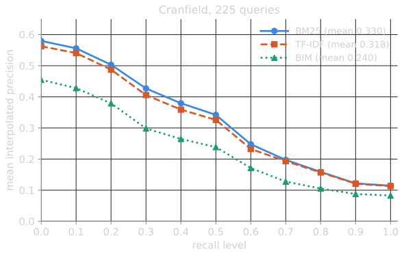
The curves show the whole trade-off at once. BM25 and TF-IDF differ only at low recall, where BM25's better top ranks show, and converge after recall 0.7. The BIM is below both everywhere. But a curve is eleven numbers, and two curves that cross cannot be ranked without deciding which part of the curve matters more, which is why single-figure measures replaced them.
Precision at k
Most users look only at the first page of results. Precision at $k$ (P@$k$) measures exactly that page: the fraction of the top $k$ results that are relevant. In the example, P@5 = 2/5 = 0.4 and P@10 = 4/10 = 0.4. It needs no knowledge of how many relevant documents exist, which makes it suitable for very large collections such as the web, where total recall is unknowable.
Its weaknesses are the other side of the same property. It ignores the order within the top $k$: a ranking with relevant documents at positions 1 and 2 has the same P@5 as one with them at 4 and 5. And it varies with the number of relevant documents. A query with only two relevant documents can never exceed P@10 = 0.2, however good the system. Averages of P@$k$ across queries mix those different ceilings.
The ceiling is not a corner case. Of Cranfield's 225 queries, 173 have fewer than 10 relevant documents (the median is 6). A perfect system would therefore score a mean P@10 of only 0.605 on Cranfield, not 1. BM25's mean P@10 of 0.234 looks poor in absolute terms; as a fraction of what was achievable, it is 0.387.
Recall at $k$, the fraction of all relevant documents found in the top $k$, is the matching measure for systems whose top $k$ results feed a later stage, such as a reranker in a multi-stage ranking. Such a system must not lose relevant documents before the reranker sees them.
R-precision
R-precision adapts the cutoff to the query. If a query has $R$ relevant documents, R-precision is the precision at rank $R$. In the example $R = 5$, so R-precision is P@5 = 0.4. A perfect system scores 1 on every query regardless of how many relevant documents it has, which removes the ceiling problem of P@$k$. It requires knowing $R$, so it needs the same judgment effort as recall.
At rank $R$, precision and recall are equal, since both are the number of relevant documents retrieved divided by $R$. For that reason R-precision is also called the break-even point. It is the only rank where they are equal (unless nothing relevant has been retrieved yet, when both are 0): if $h > 0$ relevant documents are in the top $k$, precision is $h/k$ and recall is $h/R$, which agree only when $k = R$. In the figure of precision and recall at each rank, the two curves cross at rank 5 and nowhere else. On a precision-recall plot, the break-even point is where the curve meets the diagonal $P = R$. On Cranfield, BM25's mean R-precision is 0.309, close to its MAP of 0.307.
Reciprocal rank
Some needs are satisfied by a single document, as for a known-item search, a navigational query, or a question with one answer. For these, what matters is how far down the first relevant result appears. The reciprocal rank is $1/k$, where $k$ is the rank of the first relevant document, and 0 if none is retrieved. Averaged over queries it is the mean reciprocal rank (MRR), the measure used to evaluate question answering at TREC (Voorhees, 1999). In the example the first result is relevant, so the reciprocal rank is 1. If the first relevant result had been at rank 2, it would be 0.5.
Over four queries whose first relevant results are at ranks 1, 2, and 5, and never, the reciprocal ranks are 1, 0.5, 0.2, and 0, and
$$\text{MRR} = \frac{1 + 0.5 + 0.2 + 0}{4} = 0.425.$$
MRR drops steeply with rank. Moving the first relevant result from rank 1 to rank 2 halves the score, while moving it from 9 to 10 barely changes it. That matches user behavior for single-answer needs, since few users read far down a list. A consequence is that MRR is not the reciprocal of the mean rank. For the three queries that found something, the mean rank is $(1 + 2 + 5)/3 = 2.67$, while the mean reciprocal rank is $1.7/3 = 0.567$, whose reciprocal, 1.76, is the harmonic mean of the ranks. The harmonic mean is pulled toward the small values, so one query answered at rank 1 does more for MRR than one answered at rank 50 does against it. On Cranfield, BM25 puts a relevant document first for 73 of the 225 queries and has an MRR of 0.534.
ROC curves
Classification research often uses the receiver operating characteristic (ROC) curve, which plots the true positive rate (recall) against the false positive rate, $FP/(FP + TN)$. ROC curves are rarely used in retrieval. Because nearly every document is nonrelevant, the true negatives are enormous and the false positive rate stays close to zero across the part of the ranking any user would read. The curve compresses the region that matters into a sliver near its left edge (Manning, Raghavan, and Schütze, 2008, §8.4). Precision-recall curves, which ignore true negatives, show that region clearly.
A real query shows how extreme the compression is. For BM25 on Cranfield query 2, which has 24 relevant documents among 1,400, the first 100 results contain 8 relevant and 92 nonrelevant documents. Their false positive rate is $92/1{,}376 = 0.067$, so a hundred results, far more than anyone reads, occupy the leftmost 7 percent of the ROC plot. The same hundred results span precision from 1 down to 0.08 on the precision-recall plot.
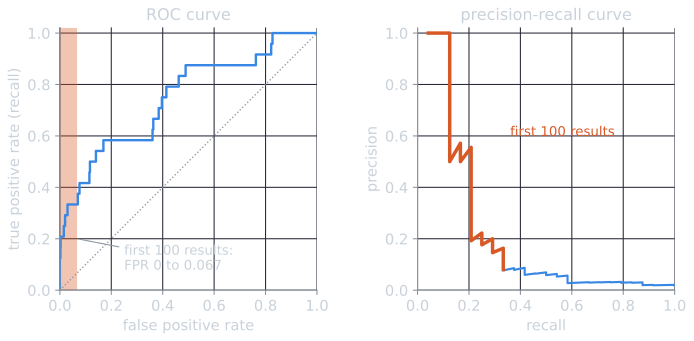
The area under the ROC curve for this query is 0.748, which sounds respectable. It is dominated by how the ranking orders the hundreds of documents nobody reads, including the 617 that share no term with the query.
Trying the measures
The demo below holds a ranking of 10 or 20 results. Clicking a result cycles its grade from 0 (not relevant) through 3 (highly relevant); any grade above 0 counts as relevant for the binary measures. The sliders set the cutoff $k$ and the number of relevant documents the system did not retrieve, which matter for recall, AP, R-precision and the ideal ranking of nDCG. The presets load the worked ranking of this article, the second query of mean average precision, and the graded example of nDCG.
Some things to try: move the relevant document at rank 9 to rank 2 and compare the change in AP with the change in P@10 (none). Set the unretrieved count to 0 and watch the interpolated curve reach recall 1. Load the all-nonrelevant preset and set the unretrieved count to 0: with no relevant documents at all, recall and nDCG are undefined, and the demo, like most tools, reports 0 (see implementing evaluation measures).
Choosing a measure
Each measure models a different user:
| Measure | Models a user who |
|---|---|
| P@$k$ | reads exactly the first $k$ results |
| Recall at $k$ | passes the top $k$ to a later stage, or must find everything within $k$ |
| R-precision | reads as many results as there are relevant documents |
| Reciprocal rank | stops at the first relevant result |
| Average precision | wants every relevant document, and values finding each one early |
| nDCG | reads with declining attention, and values some documents more than others |
No measure is correct in general. A measure should be chosen to match the task, and reporting several, as TREC does, shows whether a conclusion depends on the choice. How these measures are computed in practice, and where implementations disagree, is the subject of implementing evaluation measures.
References
- Manning, C. D., Raghavan, P., and Schütze, H. (2008). Introduction to Information Retrieval, section 8.4. Cambridge University Press.
- Voorhees, E. M. (1999). The TREC-8 question answering track report. In Proceedings of the Eighth Text REtrieval Conference (TREC-8), 77–82.