For the query jaguar habitat, a recent survey of jaguar populations by range country is more useful than a general article about big cats that mentions jaguars, and both are more useful than a page about the car. Binary judgments flatten all of this to relevant or not. Precision, recall, and average precision then reward a system equally for ranking the survey or the general article first. Most real search tasks have degrees of relevance, and a measure should reward placing the most relevant documents at the top.
Discounted cumulative gain (DCG), introduced by Järvelin and Kekäläinen (2000), does this. Its normalized form, nDCG (Järvelin and Kekäläinen, 2002), is the standard measure for web search evaluation and for most learning-to-rank research. It rests on two ideas. Documents contribute gain in proportion to how relevant they are, and the gain is discounted by how far down the ranking a document appears, because users are less likely to reach it.
The numbers in this article are computed by tools/experiments/eval_measures/worked_examples.py and cranfield_measures.py in the site's repository and rounded to three decimals.
Graded judgments
Graded collections judge documents on a small ordinal scale, for example:
| Grade | Meaning |
|---|---|
| 3 | Highly relevant: directly and fully addresses the need |
| 2 | Relevant: substantially useful |
| 1 | Marginally relevant: touches on the need |
| 0 | Not relevant |
Web search evaluations have used five-point scales, from perfect to bad. The measure works with any numeric scale.
Cumulative gain and the discount
The construction proceeds in three steps, each fixing a problem with the one before.
Cumulative gain. The simplest graded measure adds up the grades of the top $k$ results: $\mathrm{CG}@k = \sum_{i=1}^{k} \mathit{rel}_i$, where $\mathit{rel}_i$ is the grade of the document at rank $i$. It rewards retrieving highly relevant documents but ignores their order. The rankings 3, 0, 0 and 0, 0, 3 both have CG@3 = 3.
Discounting. To reward order, each gain is divided by a discount that grows with rank. The DCG of the top $k$ results is
$$\mathrm{DCG}@k = \sum_{i=1}^{k} \frac{\mathit{gain}(\mathit{rel}_i)}{\log_2(i + 1)}.$$
The discount $1/\log_2(i + 1)$ is 1 at rank 1, 0.631 at rank 2, 0.5 at rank 3, and keeps shrinking, but slowly. A highly relevant document at rank 10 still counts for about 29 percent of what it would at rank 1. The logarithm models a user whose attention fades gradually down the page rather than stopping abruptly.
The $+1$ inside the logarithm is there so that rank 1 is not divided by $\log_2 1 = 0$. Järvelin and Kekäläinen's original definition handled rank 1 differently: it applied no discount to ranks below the logarithm's base $b$, and divided by $\log_b i$ from rank $b$ on (Järvelin and Kekäläinen, 2002, §2.2, eq. 2). With $b = 2$ that leaves ranks 1 and 2 undiscounted, since $\log_2 2 = 1$. The form with $\log(1 + i)$ appears in Burges et al. (2005, §6.1, eq. 16), together with the exponential gain below; it discounts every rank after the first and is the one most tools compute.
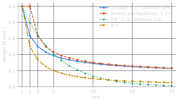
The choice of discount is a choice of user model. A logarithmic discount assumes users who keep reading, with slowly fading attention. A geometric discount, as in rank-biased precision, assumes each result is a fresh chance to stop. The figure shows how different the assumptions are in the tail.
Gain. Two forms of the gain are common:
- Linear gain, $\mathit{gain}(\mathit{rel}) = \mathit{rel}$, the form closest to Järvelin and Kekäläinen's original.
- Exponential gain, $\mathit{gain}(\mathit{rel}) = 2^{\mathit{rel}} - 1$, popularized in web search and learning-to-rank research (Burges et al., 2005). It gives grades 0, 1, 2, and 3 gains of 0, 1, 3, and 7, strongly emphasizing the most relevant documents.
Under linear gain, a grade-3 document is worth three grade-1 documents. Under exponential gain it is worth seven, and more than two grade-2 documents. Which is right depends on whether a single excellent answer is worth more than several partial ones, a question about users that the formula cannot settle.
Normalizing by the ideal ranking
DCG values cannot be compared across queries. A query with many highly relevant documents can reach a much larger DCG than one with few. Normalized DCG divides by the DCG of the best possible ranking, the ideal DCG (IDCG), obtained by sorting all the judged documents for the query by grade:
$$\mathrm{nDCG}@k = \frac{\mathrm{DCG}@k}{\mathrm{IDCG}@k}.$$
nDCG lies between 0 and 1, and equals 1 exactly when the grades of the top $k$ results match those of the ideal ranking.
A worked example
A system returns six documents with grades 3, 2, 3, 0, 1, 2. Suppose these are all the judged documents for the query, so the ideal ranking is 3, 3, 2, 2, 1, 0.
| Rank $i$ | Discount $1/\log_2(i+1)$ | System grade | Linear gain, discounted | Exponential gain, discounted |
|---|---|---|---|---|
| 1 | 1.000 | 3 | 3.000 | 7.000 |
| 2 | 0.631 | 2 | 1.262 | 1.893 |
| 3 | 0.500 | 3 | 1.500 | 3.500 |
| 4 | 0.431 | 0 | 0 | 0 |
| 5 | 0.387 | 1 | 0.387 | 0.387 |
| 6 | 0.356 | 2 | 0.712 | 1.069 |
| DCG@6 | 6.861 | 13.848 |
The ideal ranking is computed the same way:
| Rank $i$ | Discount | Ideal grade | Linear gain, discounted | Exponential gain, discounted |
|---|---|---|---|---|
| 1 | 1.000 | 3 | 3.000 | 7.000 |
| 2 | 0.631 | 3 | 1.893 | 4.417 |
| 3 | 0.500 | 2 | 1.000 | 1.500 |
| 4 | 0.431 | 2 | 0.861 | 1.292 |
| 5 | 0.387 | 1 | 0.387 | 0.387 |
| 6 | 0.356 | 0 | 0 | 0 |
| IDCG@6 | 7.141 | 14.595 |
so
| Gain | nDCG@6 |
|---|---|
| Linear | 6.861 / 7.141 = 0.961 |
| Exponential | 13.848 / 14.595 = 0.949 |
The ranking is nearly ideal. Its main fault is placing a grade-2 document above a grade-3 one at ranks 2 and 3. The exponential form penalizes that more, because it values the grade-3 document much more highly than the grade-2 one.
nDCG at each cutoff
Accumulating the rows gives DCG and IDCG at every cutoff, and their ratio:
| Cutoff $k$ | DCG@$k$ (linear) | IDCG@$k$ (linear) | nDCG@$k$ (linear) | nDCG@$k$ (exponential) |
|---|---|---|---|---|
| 1 | 3.000 | 3.000 | 1.000 | 1.000 |
| 2 | 4.262 | 4.893 | 0.871 | 0.779 |
| 3 | 5.762 | 5.893 | 0.978 | 0.959 |
| 4 | 5.762 | 6.754 | 0.853 | 0.872 |
| 5 | 6.149 | 7.141 | 0.861 | 0.876 |
| 6 | 6.861 | 7.141 | 0.961 | 0.949 |
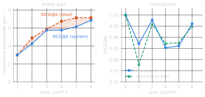
DCG@$k$, like recall at $k$, can only grow with $k$, but nDCG@$k$ can rise and fall, because the ideal ranking also gains at every cutoff. A system's nDCG@2 can be worse than its nDCG@3, as here, so a measure reported at one cutoff says little about another. At $k = 2$ the exponential gain is much harsher (0.779 against 0.871) because the ideal's second document is worth 7 under exponential gain and only 3 under linear.
Which logarithm?
Papers sometimes use the natural logarithm or base 10 in the discount. For the form $1/\log_b(i + 1)$, the base makes no difference to nDCG. Since $\log_b x = \ln x / \ln b$, every discount is multiplied by the same constant $\ln b / \ln 2$ when the base changes from 2 to $b$. DCG and IDCG are both multiplied by it, and it cancels in the ratio.
| Discount | DCG@6 (linear) | IDCG@6 (linear) | nDCG@6 linear / exponential |
|---|---|---|---|
| $1/\log_2(i+1)$ | 6.861 | 7.141 | 0.961 / 0.949 |
| $1/\ln(i+1)$ | 9.899 | 10.302 | 0.961 / 0.949 |
| $1/\log_{10}(i+1)$ | 22.792 | 23.722 | 0.961 / 0.949 |
| Järvelin and Kekäläinen, $b = 2$ | 8.097 | 8.693 | 0.932 / 0.898 |
| Järvelin and Kekäläinen, $b = 10$ | 11.000 | 11.000 | 1.000 / 1.000 |
DCG itself changes with the base, so unnormalized DCG values are comparable only with the same base. The original form is different, because its discount is not a constant multiple of anything: changing $b$ changes which ranks are undiscounted. With $b = 10$, ranks 1 to 9 are undiscounted and rank 10 is divided by $\log_{10} 10 = 1$, so the whole first page counts at face value; nDCG@6 reduces to cumulative gain divided by ideal cumulative gain, and every ordering of the six documents scores 1. The parameter $b$ was meant to model patience: Järvelin and Kekäläinen (2002, §2.2) note that a higher base means a smaller discount, for a searcher likely to examine results at least down to the base rank.
How the choices change conclusions
Linear versus exponential gain
The two gain formulas can disagree about which of two rankings is better. Take the same six judged documents and two other orderings:
| Ranking | Top three grades | nDCG@3 linear | nDCG@3 exponential |
|---|---|---|---|
| X: 3, 0, 0, 2, 2, 1 | 3, 0, 0 | 0.509 | 0.542 |
| Y: 2, 2, 1, 3, 0, 0 | 2, 2, 1 | 0.638 | 0.418 |
Under linear gain, Y's three useful documents (2 + 2 + 1) beat X's single excellent one. Under exponential gain the excellent document is worth 7 against Y's 3 + 3 + 1 spread over lower ranks, and X wins. The two rankings also swap places at nDCG@6 (0.699 and 0.708 under linear gain, 0.672 and 0.576 under exponential). Such reversals are not rare. The six documents can be ordered in 180 distinguishable ways, giving 16,110 pairs of orderings; the two gain formulas rank 1,002 of those pairs (6.2 percent) in opposite orders at nDCG@6.
Graded versus binary relevance
Graded judgments can also reverse the verdict of a binary measure. Suppose a query has one highly relevant document, three marginal ones, and two nonrelevant ones, and two systems rank them as follows:
| Ranking | AP (grades above 0 relevant) | nDCG@6 linear | nDCG@6 exponential |
|---|---|---|---|
| U: 1, 1, 1, 3, 0, 0 | 1.000 | 0.750 | 0.601 |
| V: 3, 0, 1, 1, 1, 0 | 0.804 | 0.946 | 0.971 |
U puts all four relevant documents first, so AP, which sees only relevant or not, scores it perfectly. But it makes the user read three marginal documents before the one that answers the need. V shows the answer first and pays for it with a nonrelevant document at rank 2. AP prefers U; nDCG prefers V by a wide margin. Which is right depends on the user, but only graded judgments allow the question to be asked.
On Cranfield
The Cranfield collection has graded judgments from 1 (a complete answer) to 4 (minimum interest), and the comparison in comparing ranking models uses gain $5 - \text{grade}$, so a complete answer has gain 4. Computing nDCG@10 for the same runs with binary gains instead shows how much the grades matter there:
| Model | nDCG@10, graded | nDCG@10, binary |
|---|---|---|
| BIM | 0.268 | 0.282 |
| TF-IDF | 0.356 | 0.371 |
| BM25 | 0.368 | 0.385 |
All three scores are a little lower with grades: within the top ten, the systems do not consistently place the complete answers above the documents of minimum interest. The ordering of the models does not change, and the per-query comparison of BM25 with TF-IDF changes direction on only 6 of the 225 queries. On this collection, grading changes the numbers more than the conclusions.
Properties
- Graded and top-weighted. nDCG uses the degree of relevance and the position, unlike precision at $k$, which uses neither, and AP, which uses only position.
- Focused on the top. DCG@10 needs grades only for the ten results shown. The ideal ranking still depends on knowing the best-graded documents for the topic, so incomplete judgments can distort nDCG through its denominator, as the pitfalls below explain.
- Comparable across queries, because each query is normalized to its own ideal.
Pitfalls
- Which formula? The two gain functions give different values, and implementations also differ in their discounts. Järvelin and Kekäläinen's original applied no discount to ranks up to the logarithm's base. Published nDCG values are comparable only when the formula is stated, and evaluation tools should be checked for which form they compute. trec_eval's
ndcg, for example, uses the relevance grade itself as the gain unless gains are given on the command line, divides by $\log_2(i + 1)$, and builds the ideal ranking from all the judged documents (National Institute of Standards and Technology, trec_eval source,m_ndcg.c). - What counts as ideal? The ideal ranking should be built from all the judged documents for the query, not only from those the system retrieved. Building it from the retrieved documents alone makes a system that retrieves few relevant documents look perfect. If a query's judged documents have grades 3, 3, 2, 1, 0, 0 and a system retrieves two documents graded 1 and 0, its nDCG@2 is $1/(3 + 3 \times 0.631) = 0.204$. Built from the two retrieved documents, the ideal would be 1, 0, and nDCG@2 would be 1.000.
- Queries with nothing relevant. If no judged document has a positive grade, IDCG is zero and nDCG is undefined. Tools handle this differently, by skipping such queries or by scoring them 0 or 1, which can shift averages.
The demo in evaluating ranked results computes nDCG with either gain for any assignment of grades, and its presets include this article's example.
Related measures
Expected reciprocal rank (Chapelle, Metzler, Zhang, and Grinspan, 2009) assumes a cascade model of users, who read down the ranking and stop as soon as they are satisfied, with highly relevant documents more likely to satisfy them. A highly relevant document near the top then reduces the value of everything below it, since the user has probably stopped. It generalizes reciprocal rank to graded relevance. Rank-biased precision uses a different model, in which the user stops after each result with a fixed probability, whatever the result contained. These measures, nDCG, and average precision differ mainly in their assumptions about how people read results, which is why choosing among them means choosing a model of the user.
References
- Burges, C., Shaked, T., Renshaw, E., Lazier, A., Deeds, M., Hamilton, N., and Hullender, G. (2005). Learning to rank using gradient descent. In Proceedings of ICML 2005, 89–96.
- Chapelle, O., Metzler, D., Zhang, Y., and Grinspan, P. (2009). Expected reciprocal rank for graded relevance. In Proceedings of CIKM 2009, 621–630.
- Järvelin, K., and Kekäläinen, J. (2000). IR evaluation methods for retrieving highly relevant documents. In Proceedings of SIGIR 2000, 41–48.
- Järvelin, K., and Kekäläinen, J. (2002). Cumulated gain-based evaluation of IR techniques. ACM Transactions on Information Systems, 20(4), 422–446.
- Manning, C. D., Raghavan, P., and Schütze, H. (2008). Introduction to Information Retrieval, section 8.4. Cambridge University Press.
- National Institute of Standards and Technology. trec_eval. https://github.com/usnistgov/trec_eval