Precision at a fixed cutoff answers a narrow question, and a precision-recall curve answers a broad one in too many numbers. Mean average precision (MAP) sits between them. For each query it summarizes the whole ranking in one number that rewards finding every relevant document and finding them early, and it averages that number across queries. MAP was the principal measure in TREC's ad hoc evaluations for many years, and it remains one of the most widely reported measures in the literature (Manning, Raghavan, and Schütze, 2008, §8.4).
The numbers in this article are computed by tools/experiments/eval_measures/worked_examples.py and cranfield_measures.py in the site's repository and rounded to three decimals.
Average precision for one query
For a single query with $R$ relevant documents, average precision (AP) is the average, over the relevant documents, of the precision at the rank where each one is retrieved. A relevant document that is never retrieved contributes a precision of zero. Writing $k_j$ for the rank of the $j$-th relevant document retrieved,
$$\text{AP} = \frac{1}{R} \sum_{j=1}^{R} P@k_j, \qquad \text{with } P@k_j = 0 \text{ if the } j\text{-th relevant document is not retrieved.}$$
The same quantity can be written as a sum over every rank of the ranking, which is how it is usually computed. Let $\mathit{rel}(k)$ be 1 if the document at rank $k$ is relevant and 0 otherwise, and $n$ the length of the ranking. Then
$$\text{AP} = \frac{1}{R} \sum_{k=1}^{n} P@k \cdot \mathit{rel}(k).$$
The factor $\mathit{rel}(k)$ switches off the nonrelevant ranks, leaving one term per retrieved relevant document. Missing relevant documents contribute nothing to the sum but still count in $R$.
Take the ranking from evaluating ranked results: 5 relevant documents, retrieved at ranks 1, 3, 6, and 9, with the fifth never retrieved.
| Relevant document | Rank | Precision at that rank | Contribution $P@k_j / R$ |
|---|---|---|---|
| 1st | 1 | 1/1 = 1.000 | 0.200 |
| 2nd | 3 | 2/3 = 0.667 | 0.133 |
| 3rd | 6 | 3/6 = 0.500 | 0.100 |
| 4th | 9 | 4/9 = 0.444 | 0.089 |
| 5th | not retrieved | 0 | 0 |
$$\text{AP} = \frac{1.000 + 0.667 + 0.500 + 0.444 + 0}{5} = 0.522.$$
The division is by $R = 5$, the number of relevant documents, not by the 4 that were retrieved. Dividing by 4 would give 0.653 and would reward the system for having missed a relevant document. This is a common mistake in hand-written implementations, and it makes AP depend on how deep the ranking was cut.
AP as an area
Each relevant document advances recall by exactly $1/R$, and its contribution to AP is its precision times $1/R$. That is the area of a rectangle of width $1/R$ (the recall step) and height $P@k_j$ (the precision at the step). AP is the total area of these rectangles, which is the area under the precision-recall curve when precision between recall steps is held at its value at the relevant document that ends the step.
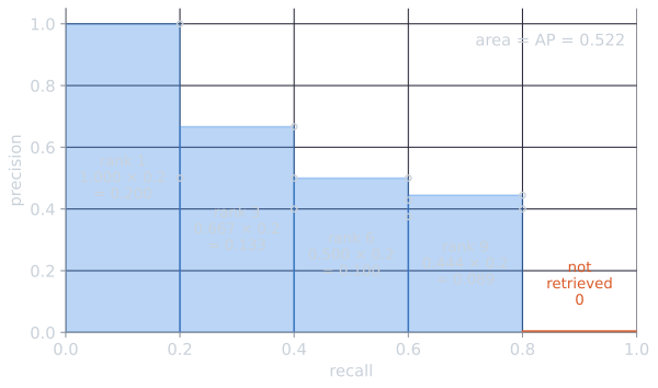
The picture explains several properties at once. A missed relevant document is an empty strip on the recall axis, so it costs AP $1/R$ times whatever precision it would have had. A nonrelevant document never adds area but lowers the height of every rectangle to its right. And because the rectangles are uninterpolated, AP differs from the area under the interpolated curve: the 11-point average of the same ranking is 0.566, higher because interpolation raises each point to the best precision further along.
Averaging over queries
MAP is the mean of AP over a set of queries $Q$:
$$\text{MAP} = \frac{1}{\lvert Q \rvert} \sum_{q \in Q} \text{AP}(q).$$
A second query has 3 relevant documents, retrieved at ranks 2, 5, and 8. Its AP is $(1/2 + 2/5 + 3/8)/3 = (0.500 + 0.400 + 0.375)/3 = 0.425$. The MAP over the two queries is $(0.522 + 0.425)/2 = 0.474$.
Each query counts equally, however many relevant documents it has. This is a macro-average, and it reflects the view that each information need matters as much as any other. A query with 200 relevant documents does not dominate one with 2.
MAP on a real collection
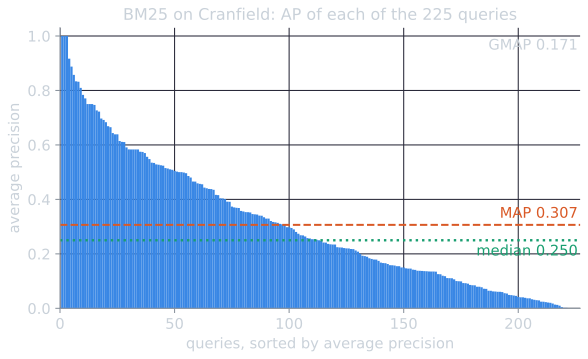
Two queries hide how much AP varies. On the Cranfield collection, the BM25 run from comparing ranking models has a MAP of 0.307 over 225 queries, and the individual APs span the whole range.
| Statistic of per-query AP (BM25, Cranfield) | Value |
|---|---|
| Mean (MAP) | 0.307 |
| Median | 0.250 |
| Lower and upper quartiles | 0.111 and 0.483 |
| Queries with AP = 1 | 3 |
| Queries with AP = 0 | 4 |
| Queries with AP below 0.1 | 53 |
| Share of the total AP from the best quarter of queries | 0.527 |
The best quarter of the queries contributes more than half of the sum that MAP averages. A change to the system that helps those queries a little can therefore move MAP as much as one that rescues many hard queries, which is the problem the geometric mean below addresses. The spread also matters for comparing systems. BM25 and TF-IDF differ in MAP by 0.012 on Cranfield, while the middle half of BM25's per-query APs alone spans 0.37. Differences between systems are small next to differences between queries, which is why comparisons need significance tests over the per-query values rather than a look at the two means.
Neither is the spread explained by how many relevant documents a query has. Cranfield queries have between 1 and 39 relevant documents, and the correlation between that count and BM25's AP is −0.10. Some queries are hard for reasons the count does not capture, such as vocabulary that the relevant documents do not share.
What AP rewards
AP is top-heavy: a relevant document contributes more when it is ranked earlier, and moving a relevant document up affects the score more near the top of the ranking than near the bottom. In the example:
| Change to the ranking | AP |
|---|---|
| Original | 0.522 |
| Swap ranks 2 and 3, moving the 2nd relevant document from 3 to 2 | 0.589 |
| Swap ranks 9 and 10, moving the 4th relevant document from 9 to 10 | 0.513 |
A one-position move changes AP by 0.067 near the top of this ranking and by only 0.009 near the bottom.
The formula shows why. Suppose the $j$-th relevant document moves from rank $k$ to rank $k - 1$, swapping places with a nonrelevant document. The relevant documents before it are unaffected, and so are those after it, since the number of documents and the number of relevant documents above each of them do not change. Only the moved document's own precision changes, from $j/k$ to $j/(k-1)$. So
$$\Delta\text{AP} = \frac{1}{R}\left(\frac{j}{k - 1} - \frac{j}{k}\right) = \frac{j}{R\,k\,(k - 1)}.$$
For a given $j$ the gain falls off as $1/k^2$. Across a ranking, where $j/k$ is roughly the precision at that depth, it is about $P@k/(Rk)$: smaller deeper down both because $k$ is larger and because precision has usually fallen. For each relevant document of the example in turn:
| Move | $j$ | $k$ | $\Delta$AP $= j/(5k(k-1))$ | New AP |
|---|---|---|---|---|
| 2nd relevant, rank 3 to 2 | 2 | 3 | 0.067 | 0.589 |
| 3rd relevant, rank 6 to 5 | 3 | 6 | 0.020 | 0.542 |
| 4th relevant, rank 9 to 8 | 4 | 9 | 0.011 | 0.533 |
The same reasoning explains why evaluation depth matters little once it is deep. If the fifth relevant document of the example had been retrieved at rank 11, it would add $(5/11)/5$ and AP would be 0.613; at rank 20, 0.572; at rank 100, 0.532; at rank 1,000, 0.523. A relevant document found very deep is worth almost nothing. TREC runs conventionally list 1,000 documents per topic, and anything beyond that depth counts as not retrieved; the calculation shows that the truncation changes AP very little.
AP also approximates the area under the uninterpolated precision-recall curve, as the figure above shows, so a single number summarizes the entire curve. Buckley and Voorhees (2000) found MAP to be among the most stable measures for comparing systems: it ranks systems consistently across different topic sets, with about half the error rate of precision at 30 documents. That combination is why it became standard.
Weaknesses
- It needs complete judgments. AP depends on $R$, the number of relevant documents, and on knowing which retrieved documents are relevant. With incomplete judgments, unjudged relevant documents are counted as nonrelevant and lower the score. In the example, if the document at rank 2 had never been judged but was in fact relevant, the true AP would be computed with $R = 6$ and relevant documents at ranks 1, 2, 3, 6 and 9: $(1 + 1 + 1 + 4/6 + 5/9)/6 = 0.704$, against the 0.522 reported. Measures designed for incomplete judgments are discussed in relevance judgments, pooling, and agreement.
- It is hard to explain to users. P@10 has an obvious meaning, while AP does not correspond to any simple thing a person experiences. Robertson (2008) gave it one: AP is the expected precision at the rank of a relevant document chosen at random, for a user who stops reading at that document. That is a coherent model of a user who wants every relevant document, but not of a user who wants one good answer.
- It treats relevance as binary. A highly relevant document and a marginally relevant one count the same. nDCG uses graded relevance.
Robertson's interpretation can be checked on the example. Pick one of the five relevant documents at random, each with probability 1/5, and record the precision at its rank, or 0 if it was not retrieved. The five possible outcomes are 1.000, 0.667, 0.500, 0.444, and 0, and their expected value is $2.611/5 = 0.522$, which is AP. The definition of AP is exactly this expectation; the interpretation lies in seeing the random choice as a model of where users stop.
The geometric mean
The arithmetic mean lets large gains on easy queries hide failures on hard ones. Consider two systems on four queries:
| Query 1 | Query 2 | Query 3 | Query 4 | MAP | GMAP | |
|---|---|---|---|---|---|---|
| System A | 0.40 | 0.40 | 0.40 | 0.02 | 0.305 | 0.189 |
| System B | 0.38 | 0.38 | 0.38 | 0.20 | 0.335 | 0.324 |
System B is slightly worse on three queries and much better on the fourth, where System A nearly fails. MAP prefers B by a little. The geometric mean average precision (GMAP), the geometric mean of the per-query AP values, prefers B by a lot, because a geometric mean is dominated by its smallest values. GMAP was introduced in TREC's Robust track, whose aim was to improve the worst-performing queries rather than the average (Voorhees, 2005), and Robertson (2006) later analyzed its properties.
The geometric mean is the exponential of the mean logarithm,
$$\text{GMAP} = \exp\left(\frac{1}{\lvert Q \rvert} \sum_{q \in Q} \log \text{AP}(q)\right),$$
which shows why it rewards gains on hard queries. On the log scale, raising AP from 0.02 to 0.20 is the same improvement as raising it from 0.1 to 1: a tenfold increase. Raising it from 0.40 to 0.42 is a small one wherever it happens. An AP of zero makes the logarithm undefined and the geometric mean zero, so in practice each AP is kept away from zero before taking the logarithm. trec_eval's gm_map replaces each AP by the larger of it and 0.00001 (National Institute of Standards and Technology, trec_eval source, m_gm_map.c); other implementations add a small constant. The choice of floor changes the value of GMAP whenever a query scores zero.
On Cranfield, with trec_eval's floor:
| Model | MAP | GMAP |
|---|---|---|
| BIM | 0.220 | 0.110 |
| TF-IDF | 0.294 | 0.166 |
| BM25 | 0.307 | 0.171 |
GMAP is about half of MAP for every model, because the many queries with AP below 0.1 weigh heavily on the log scale. BM25 leads TF-IDF by 4.2 percent in MAP and by 3.1 percent in GMAP (computed before rounding), so on this collection its advantage comes slightly more from queries that were already going well.
Other user models
Moffat and Zobel (2008) argued that a measure should be based on an explicit model of how users read. Their rank-biased precision assumes that after each result a user continues to the next with a fixed probability $p$, and scores a ranking by the expected rate at which the user encounters relevant documents. Under that model the user reaches rank $i$ with probability $p^{i-1}$, so the weight of each rank falls geometrically, much faster in the tail than AP's or nDCG's (the nDCG article plots these weights side by side). Unlike AP, it does not need to know the total number of relevant documents, and the parameter $p$ states directly how patient the user is assumed to be. nDCG, described next, is another measure built on a model of declining attention.
The demo in evaluating ranked results computes AP alongside the other measures for any ranking, and shows the top-heaviness directly: moving a relevant document up one rank near the top changes AP far more than the same move near the bottom.
References
- Buckley, C., and Voorhees, E. M. (2000). Evaluating evaluation measure stability. In Proceedings of SIGIR 2000, 33–40.
- Manning, C. D., Raghavan, P., and Schütze, H. (2008). Introduction to Information Retrieval, section 8.4. Cambridge University Press.
- Moffat, A., and Zobel, J. (2008). Rank-biased precision for measurement of retrieval effectiveness. ACM Transactions on Information Systems, 27(1), article 2.
- National Institute of Standards and Technology. trec_eval. https://github.com/usnistgov/trec_eval
- Robertson, S. (2006). On GMAP: And other transformations. In Proceedings of CIKM 2006, 78–83.
- Robertson, S. (2008). A new interpretation of average precision. In Proceedings of SIGIR 2008, 689–690.
- Voorhees, E. M. (2005). The TREC robust retrieval track. SIGIR Forum, 39(1), 11–20.