Every measure in this topic is computed against relevance judgments: someone's decision, for a given information need, about which documents are relevant. The judgments are the most expensive part of a test collection and the most fragile. A collection of a million documents and fifty topics would require fifty million decisions to judge exhaustively. At a few seconds each, that would take a single assessor decades. And as relevance explains, two careful assessors judging the same documents often disagree. This article covers how collections cope with both problems: pooling to reduce the number of judgments, and agreement statistics to measure how much the judgments can be trusted.
Who judges, and how
In TREC, each topic is usually written by the assessor who later judges it, so that the person deciding relevance is the person whose need the topic describes. Assessors judge each document against the topic's narrative, which states what counts as relevant (see test collections). They see documents one at a time, typically without knowing which system retrieved them or how highly, so that their judgments are not influenced by the systems being compared.
Judgments are usually binary. Graded judgments, which nDCG is designed to use, cost more, since assessors must also decide how relevant each document is, and agreement between assessors is lower for fine distinctions.
Pooling
Exhaustive judging is impossible for a large collection, but most documents are obviously nonrelevant to any given topic. Pooling judges only the documents some system found worth ranking highly. For each topic:
- Collect the rankings submitted by all participating systems.
- Take the top $k$ documents from each ranking, typically $k = 100$ in TREC's ad hoc tracks.
- Judge the union of those documents, the pool.
- Treat every document outside the pool as nonrelevant.
Pools overlap heavily, since good systems tend to find the same documents, so a pool is much smaller than the number of systems times $k$. With three systems contributing their top five documents,
System A: 3, 7, 12, 5, 9
System B: 7, 3, 15, 22, 5
System C: 12, 40, 3, 7, 18
the pool is {3, 5, 7, 9, 12, 15, 18, 22, 40}: nine documents to judge instead of fifteen. With dozens of systems and $k = 100$, a TREC pool typically held on the order of a thousand or two documents per topic, out of hundreds of thousands or millions.
Pooling simulated on Cranfield
Cranfield's judgments were made by screening every document against every query (see test collections), so it can show what a pool would have found. The script tools/experiments/cranfield/pooling.py runs twelve systems over the 225 queries, chosen to differ the way the participants of a TREC track differ: BM25 with several parameter settings, with and without stemming and stop-word removal; TF-IDF cosine with and without stemming; query likelihood with Dirichlet smoothing, with and without stemming; the binary independence model; and two deliberately weak systems, coordination-level matching (the number of query terms a document contains) and raw term-frequency sums. Their MAP on the full judgments ranges from 0.311 down to 0.029. For each depth $k$, the pool for a query is the union of the twelve top-$k$ lists, and a relevant document counts as found if it is in the pool.
| Depth $k$ | Documents to judge per query | Share of 12 × $k$ | Share of the collection | Relevant documents found | Best single run alone |
|---|---|---|---|---|---|
| 1 | 3.8 | 32% | 0.3% | 11% | 5% |
| 5 | 17.8 | 30% | 1.3% | 34% | 23% |
| 10 | 33.7 | 28% | 2.4% | 45% | 34% |
| 20 | 63.8 | 27% | 4.6% | 56% | 46% |
| 50 | 148.4 | 25% | 10.6% | 70% | 60% |
| 100 | 277.1 | 23% | 19.8% | 80% | 71% |
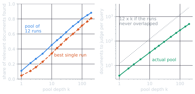
Three things stand out. Overlap is heavy: twelve runs to depth 100 propose 1,200 documents per query, but only 277 are distinct, because the systems agree on most of what they rank highly. Pooling also beats any one system. At every depth the union finds between 6 and 11 percentage points more of the relevant documents than the best run's list of the same depth, because different systems fail on different relevant documents. And the pool is far from complete at practical depths. At depth 100 it judges a fifth of the collection and still misses a fifth of the relevant documents; 16 relevant pairs were not in any run's top 1,000. Cranfield's queries are long and its documents are short abstracts, so the exact numbers do not transfer to TREC. The lesson does: a pool is a sample of the relevant documents, not a census.
Is pooling reliable?
Pooling misses relevant documents that no participating system ranked highly, and it treats them as nonrelevant. Zobel (1998) estimated that TREC pools missed a substantial fraction of relevant documents for many topics. He also found that the comparisons between systems remained reliable. Measured recall was therefore overestimated for every system, but the missing documents rarely changed which system ranked above which. For systems that took part in building the pool, pooled judgments support comparison well.
Two risks remain:
- Reusability. A new system, built after the pool, may retrieve relevant documents nobody judged, and it will be scored as if they were nonrelevant. The more different the new system is from the original participants, the more it is underestimated. Neural rankers evaluated on collections pooled from older term-matching systems are a contemporary example.
- Bias at scale. In very large collections, pools can be dominated by documents that contain the topic's title words, because most systems rank such documents highly. Relevant documents that use other vocabulary are then underrepresented. Buckley, Dimmick, Soboroff, and Voorhees (2007) found this bias in pools for large collections and showed it can distort comparisons.
Both effects on Cranfield
The Cranfield simulation can show both the reassuring result and the risk, because the full judgments say what the right answer is.
To compare two orderings of systems, the standard statistic is Kendall's $\tau$. Take every pair of systems, $\binom{12}{2} = 66$ pairs for twelve systems, and call a pair concordant if both orderings put the same system first and discordant otherwise. Then
$$\tau = \frac{\text{concordant pairs} - \text{discordant pairs}}{\text{all pairs}}.$$
It is 1 for identical orderings, −1 for reversed ones, and each swapped pair out of 66 lowers it by $2/66 \approx 0.03$.
Scores rise, the order holds. Judged against the depth-10 pool of all twelve runs, with unpooled documents counted as nonrelevant, every system's MAP rises: BM25 goes from 0.307 to 0.439. The pool's missing relevant documents disappear from the denominator of recall, which is the overestimate Zobel described. Yet the ordering of the twelve systems has $\tau = 0.97$ against the true ordering (one swapped pair), and 1.0 at depth 20. A leave-one-out test asks what would have happened to each system had it not contributed: its unique documents are removed from the pool before it is scored. The largest drop in MAP was 0.0065, for the weakest run, which contributed the most documents nobody else retrieved; one system lost a place at depth 10, and none moved at depths 20 or 50.
A new kind of system is underrated. Leave-one-out is mild here because each of the twelve has relatives in the pool. The risk appears when the pool comes from one family. In the next experiment only the four stemmed BM25 variants built the depth-10 pool, and the other eight were scored against it as if they were later systems:
| System | True MAP | MAP against the BM25 pool | Top 10 unjudged | Rank: true → pool |
|---|---|---|---|---|
| BM25 $k_1 = 3$ (in pool) | 0.311 | 0.467 | 0% | 1 → 1 |
| BM25 (in pool) | 0.307 | 0.463 | 0% | 2 → 3 |
| BM25, stop words kept (in pool) | 0.306 | 0.464 | 0% | 3 → 2 |
| TF-IDF | 0.294 | 0.438 | 13% | 4 → 4 |
| BM25 unstemmed | 0.282 | 0.420 | 21% | 5 → 5 |
| Query likelihood | 0.277 | 0.419 | 16% | 6 → 6 |
| TF-IDF unstemmed | 0.274 | 0.398 | 29% | 7 → 8 |
| BM25 $b = 0$ (in pool) | 0.271 | 0.407 | 0% | 8 → 7 |
| Query likelihood unstemmed | 0.255 | 0.377 | 32% | 9 → 9 |
| BIM | 0.220 | 0.323 | 23% | 10 → 10 |
| Coordination | 0.172 | 0.258 | 38% | 11 → 11 |
| Raw TF | 0.029 | 0.037 | 88% | 12 → 12 |
The pool found 39 percent of the relevant documents. BM25 with $b = 0$, a member, is truly worse than unstemmed TF-IDF, an outsider, but the pool ranks it higher. Overall $\tau = 0.94$ (two swapped pairs); with a depth-5 pool it falls to 0.88. The unjudged column is the warning sign recommended in test collections: the members have no unjudged documents in their top ten, while the outsiders have 13 to 38 percent, and the weakest has 88 percent. A system with a third of its top ten unjudged is being scored partly on a guess. Cranfield's runs are all variations on term matching, so the bias here is small; a system that differs more from the pool's contributors, such as a neural ranker scored on a pool built from term-matching systems, has more room to be underrated.
Measures for incomplete judgments
When many retrieved documents are unjudged, measures can avoid treating them as nonrelevant. bpref (Buckley and Voorhees, 2004) scores a ranking using only the judged documents, counting how often judged nonrelevant documents are ranked above judged relevant ones. Inferred average precision (Yilmaz and Aslam, 2006) estimates average precision from a random sample of the pool rather than the whole pool, which makes judging cheaper and gives unbiased estimates. A simpler safeguard, recommended in test collections, is to report the fraction of each system's top results that is unjudged.
Measuring agreement
If judgments depend on the judge, their reliability can be measured by having two assessors judge the same documents and comparing the results. Simple percentage agreement is misleading, because two judges who both mark nearly everything nonrelevant will agree most of the time by chance. The kappa statistic corrects for chance:
$$\kappa = \frac{P(A) - P(E)}{1 - P(E)},$$
where $P(A)$ is the proportion of documents on which the judges agree and $P(E)$ is the proportion on which they would agree by chance, given how often each says "relevant". Kappa is 1 for perfect agreement, 0 for agreement no better than chance, and negative for systematic disagreement.
Where the formula comes from
Suppose judge 1 calls a fraction $p_1$ of the documents relevant and judge 2 a fraction $p_2$, and suppose each decides without regard to the other, as if flipping biased coins. They agree when both say relevant, with probability $p_1 p_2$, or both say nonrelevant, with probability $(1 - p_1)(1 - p_2)$. So the agreement expected by chance is
$$P(E) = p_1 p_2 + (1 - p_1)(1 - p_2).$$
Agreement beyond chance is then $P(A) - P(E)$. The most there could be is $1 - P(E)$, reached when the judges agree on every document. Kappa is the ratio of the two: the share of the possible above-chance agreement that the judges achieved. Reading it this way explains its range. A pair who agree exactly as often as independent coin-flippers would score 0, whatever their raw agreement, and only a pair who disagree more often than chance can score below 0.
A worked example
Manning, Raghavan, and Schütze (2008, §8.5) give the judgments of two assessors on 400 documents:
| Judge 2: relevant | Judge 2: nonrelevant | Total | |
|---|---|---|---|
| Judge 1: relevant | 300 | 20 | 320 |
| Judge 1: nonrelevant | 10 | 70 | 80 |
| Total | 310 | 90 | 400 |
The judges agree on $300 + 70 = 370$ documents, so $P(A) = 370/400 = 0.925$.
For chance agreement, the textbook pools the two judges' marginals. Of the 800 judgments made in total, $320 + 310 = 630$ were "relevant", so $P(\text{relevant}) = 630/800 = 0.7875$ and $P(\text{nonrelevant}) = 0.2125$. Two independent judges with those rates would agree with probability
$$P(E) = 0.7875^2 + 0.2125^2 = 0.6653.$$
Then
$$\kappa = \frac{0.925 - 0.6653}{1 - 0.6653} = 0.776.$$
The judges agreed on 92.5 percent of documents, but much of that is expected from chance, because both judged most documents relevant. Kappa reports the agreement beyond chance. Manning, Raghavan, and Schütze describe values above 0.8 as good agreement, 0.67 to 0.8 as fair, and below 0.67 as a dubious basis for evaluation. By that scale this pair's agreement is fair. They note that agreement on TREC and similar collections has generally fallen in the fair range. (A common variant, Cohen's kappa, computes chance agreement from each judge's own rates rather than pooled rates. The two give similar values when the judges' rates are similar.)
The pooled version uses one rate $p$ for both judges in the formula of the previous section, $P(E) = p^2 + (1 - p)^2$. Cohen's version uses each judge's own rate, here $p_1 = 320/400 = 0.8$ and $p_2 = 310/400 = 0.775$:
$$P(E) = 0.8 \times 0.775 + 0.2 \times 0.225 = 0.62 + 0.045 = 0.665, \qquad \kappa = \frac{0.925 - 0.665}{1 - 0.665} = 0.776.$$
The two rates are close, so the answers agree to three decimals. They part company when the judges' rates differ. If judge 1 marks 70 of 400 documents relevant and judge 2 marks 10, all 10 of them among judge 1's 70, then $P(A) = 340/400 = 0.85$; Cohen's kappa is 0.216 and the pooled kappa 0.167. Pooling the rates assumes the judges share one underlying tendency to say "relevant", so a difference in their rates counts as disagreement. Cohen's version takes each judge's tendency as given and measures agreement only beyond it. (These numbers, and all others in this section, are computed in tools/experiments/cranfield/pooling.py.)
High agreement, low kappa
Kappa depends strongly on how common relevant documents are. Keep the same raw agreement as the textbook's pair, 370 of 400, but suppose relevant documents are rare:
| Judge 2: relevant | Judge 2: nonrelevant | Total | |
|---|---|---|---|
| Judge 1: relevant | 10 | 15 | 25 |
| Judge 1: nonrelevant | 15 | 360 | 375 |
| Total | 25 | 375 | 400 |
Now $P(A) = 0.925$ as before, but each judge says "relevant" for only $p = 25/400 = 0.0625$ of the documents, so
$$P(E) = 0.0625^2 + 0.9375^2 = 0.0039 + 0.8789 = 0.8828, \qquad \kappa = \frac{0.925 - 0.8828}{1 - 0.8828} = 0.36.$$
The same 92.5 percent agreement now earns a kappa in the "dubious" range, and rightly. Of the 40 documents that either judge called relevant, the judges agreed on only 10. Almost all of their agreement is on obviously nonrelevant documents, which any two judges would agree on. Retrieval judgments usually look like this second table, since most documents are nonrelevant to most topics, which is why raw agreement is never reported alone.
Substituting one assessor for another
As relevance describes, Voorhees (2000) found that substituting one assessor's judgments for another's changed systems' scores substantially but rarely changed the order of systems. Moderate agreement is enough for comparative evaluation, which is what test collections are for.
Why should that be? A simulation on Cranfield shows the mechanism, and its limit. The script creates a second assessor for every query by rejudging the documents. It keeps each of the original assessor's relevant documents with a probability that falls with the grade (0.9 for grade 1, 0.8 for grade 2, 0.6 for grade 3, 0.4 for grade 4), on the assumption that marginal documents are where judges disagree, and it marks as relevant 4 percent of the nonrelevant documents in the depth-20 pool. These numbers are assumptions, chosen so that the overlap between the two assessors' relevant sets, the size of their intersection divided by the size of their union, is about 0.45, inside the range of 0.42 to 0.49 that Voorhees reported for pairs of TREC-4 assessors. Over 30 seeds (medians, with interquartile ranges):
| Quantity | Median | IQR |
|---|---|---|
| Overlap of relevant sets | 0.45 | 0.45 to 0.46 |
| Cohen's kappa over the pooled documents | 0.60 | 0.59 to 0.61 |
| Mean absolute change in a system's MAP | 0.067 | 0.065 to 0.072 |
| The same, relative to the system's MAP | 31% | 29% to 33% |
| Kendall's $\tau$ between the two orderings of the 12 systems | 0.91 | 0.91 to 0.94 |
| Pairs of systems that swap, out of 66 | 3 | 2 to 3 |
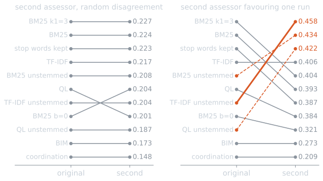
Scores move a lot, about a third of their value, but the ordering hardly moves. The reason is that random disagreement affects every system in roughly the same way. Every system loses some of the documents it found and gains credit for some it ranked highly, and a system that is better at finding the first assessor's relevant documents is, on average, also better at finding the second's. Only systems whose scores were nearly tied trade places.
The right-hand panel shows the limit. The second assessor there is equally plausible by the agreement statistics, with an overlap of 0.48 and a kappa of 0.63, both slightly higher than for the random assessor. But this assessor's extra relevant documents are drawn from the top five of one particular run, unstemmed TF-IDF, as if the assessor shared that system's notion of what the query is about. Kendall's $\tau$ falls to 0.42, and the favoured run goes from seventh to first in all 30 seeds. Agreement statistics measure how much two assessors disagree, not whether the disagreement is correlated with the systems being compared, and only the second kind distorts comparisons. Voorhees's finding is that, for TREC's human assessors, the disagreement behaved like the left panel. It is a finding about those assessors, not a guarantee, and it is the reason the model-generated judgments below need care.
Cheaper judges
Since judgments are the bottleneck, cheaper sources have been studied extensively.
Crowdsourcing hires many non-expert workers through online platforms to judge documents, usually with several workers per document and quality checks such as documents with known answers. Alonso, Rose, and Stewart (2008) showed that crowdsourced judgments could be collected quickly and cheaply, with quality adequate for many purposes when aggregated across workers.
Large language models are the most recent candidate. Given a topic and a document, a model can be prompted to produce a relevance grade. Thomas, Spielman, Craswell, and Mitra (2024) reported that carefully prompted models produced judgments that agreed with searchers' own preferences about as well as human annotators did, and Faggioli and colleagues (2023) examined the opportunities and risks. The central risk is circularity. If the systems being evaluated are themselves built on language models, judgments from a similar model may favor them for reasons unrelated to relevance. Model-generated judgments are therefore usually validated against a sample of human judgments before they are trusted.
References
- Alonso, O., Rose, D. E., and Stewart, B. (2008). Crowdsourcing for relevance evaluation. SIGIR Forum, 42(2), 9–15.
- Buckley, C., Dimmick, D., Soboroff, I., and Voorhees, E. (2007). Bias and the limits of pooling for large collections. Information Retrieval, 10(6), 491–508.
- Buckley, C., and Voorhees, E. M. (2004). Retrieval evaluation with incomplete information. In Proceedings of SIGIR 2004, 25–32.
- Faggioli, G., Dietz, L., Clarke, C. L. A., et al. (2023). Perspectives on large language models for relevance judgment. In Proceedings of ICTIR 2023, 39–50.
- Manning, C. D., Raghavan, P., and Schütze, H. (2008). Introduction to Information Retrieval, section 8.5. Cambridge University Press.
- Thomas, P., Spielman, S., Craswell, N., and Mitra, B. (2024). Large language models can accurately predict searcher preferences. In Proceedings of SIGIR 2024, 1930–1940.
- Voorhees, E. M. (2000). Variations in relevance judgments and the measurement of retrieval effectiveness. Information Processing and Management, 36(5), 697–716.
- Yilmaz, E., and Aslam, J. A. (2006). Estimating average precision with incomplete and imperfect judgments. In Proceedings of CIKM 2006, 102–111.
- Zobel, J. (1998). How reliable are the results of large-scale information retrieval experiments? In Proceedings of SIGIR 1998, 307–314.