Twenty-one measurements of an unknown quantity $y$ at inputs $x = -1.0, -0.9, \dots, 1.0$ lie on a smooth curve. Ordinary regression begins by choosing a form for that curve, say a straight line $y = a + bx$ or a parabola $y = a + bx + cx^2$, and then finds the coefficients that fit best. If the chosen form is wrong, the fit is poor and the analyst tries another form by hand. Symbolic regression removes the first step: it searches for the formula itself, its structure and its constants together, among all expressions that can be built from a given set of operations (Poli, Langdon and McPhee, 2008, §12.2). For the 21 points above the answer might be $x^2 + x + 1$, and a symbolic regression system should be able to say so in those terms.
Symbolic regression was one of the earliest applications of genetic programming (GP) (Koza, 1992), and it continues to be widely studied (Poli, Langdon and McPhee, 2008, §12.2). Expressions are represented as program trees; the tree for $x^2 + x + 1$ is (+ (* x x) (+ x 1)) in prefix notation. A population of random trees is improved by selection, subtree crossover and mutation, as described in initialization and variation in genetic programming. This article covers what is particular to the regression setting: how fitness is measured, where constants come from, what a run produces, and what a formula that fits the data does elsewhere.
Two classic problems
One of Koza's (1992) introductory examples is a quartic polynomial, $x^4 + x^3 + x^2 + x$, sampled at 20 points in $[-1, 1]$. The function set was $\{+, -, \times, \%, \sin, \cos, \exp, \mathrm{rlog}\}$, where $\%$ is protected division and rlog a protected logarithm, and the only terminal was $x$. The transcendental functions are not needed; they make the point that GP is given a vocabulary, not a form, and must find out which words to use. Each sample point is a fitness case. Raw fitness was the sum over the 20 cases of the absolute error, and a case counted as a hit when the error was below 0.01.
The course's example, taken from Poli, Langdon and McPhee (2008, ch. 4), is the quadratic $x^2 + x + 1$ on $[-1, 1]$:
| Preparatory step | Choice |
|---|---|
| Terminal set | $x$ and ephemeral random constants in $[-5, 5]$ |
| Function set | $+$, $-$, $\times$, $\%$ (protected division) |
| Fitness | sum of absolute errors at $x = -1.0, -0.9, \dots, 1.0$ (21 cases) |
| Termination | a program with error below 0.1 |
The target can be written with these primitives, so the set is sufficient in the sense of program trees in genetic programming. Poli, Langdon and McPhee walk through one generation of a population of four to show the mechanics. The best initial program, $x + 1$, has error 7.7, which is easy to check: the difference from the target is $x^2$, and $\sum x^2$ over the 21 points is $2(0.01 + 0.04 + \dots + 1) = 7.7$. Crossover then combines the $x^2$ of a second parent, $x^2 + 1$, with the $x + 1$ of the first to produce the target in one step. A run of realistic size takes longer, as the experiment below shows.
Fitness on sample points
Fitness in symbolic regression is a distance between the program's outputs and the data, computed at the fitness cases. With $n$ cases $(x_i, y_i)$ and a program $p$, the two common measures are the sum of absolute errors and the mean squared error:
$$E_{\mathrm{abs}}(p) = \sum_{i=1}^{n} \lvert p(x_i) - y_i \rvert, \qquad E_{\mathrm{MSE}}(p) = \frac{1}{n} \sum_{i=1}^{n} \bigl(p(x_i) - y_i\bigr)^2.$$
For evenly spaced points, $E_{\mathrm{abs}}$ divided by $n$ approximates the average gap between the two curves over the interval, which is why Poli, Langdon and McPhee (2008, §4.1) describe it as roughly proportional to the area between them. Lower is better, and zero means the program passes through every point.
The hits criterion is a second, coarser measure. A program scores a hit on a case when its error there is below a tolerance, 0.01 in Koza's problem, and a run is usually called successful when one program hits every case. Hits are useful for reporting, because "solved in 14 of 30 runs" is easier to read than a distribution of error sums, but they define success relative to the sample. A program that hits all 20 cases has been checked at 20 points and nowhere else.
That is the central limitation of sample-based fitness. Fitness says nothing about the program's behavior between the cases or outside their range. A protected division whose divisor crosses zero between two cases creates a pole that the cases never see, as the article on program trees shows with (% 1 (- x 0.3)). Keijzer (2003) addressed this with interval arithmetic, which checks that an expression is defined over the whole range spanned by the data so that ordinary division can replace the protected one, together with linear scaling, which rescales each program's output to $a + b\,p(x)$ with the slope and intercept that minimize the squared error, computed in closed form. He reported greatly improved predictive performance and reliability on 15 symbolic regression problems.
Linear scaling worked through
The closed form for the scaling comes from ordinary least squares. For a program $p$ with outputs $p_i = p(x_i)$, choose $a$ and $b$ to minimize
$$S(a, b) = \sum_{i=1}^{n} \bigl(y_i - a - b\,p_i\bigr)^2.$$
Setting $\partial S / \partial a = -2 \sum_i (y_i - a - b\,p_i) = 0$ gives $a = \bar{y} - b\,\bar{p}$, where bars denote means over the fitness cases: the scaled program must pass through the point of means. Substituting this $a$ and setting $\partial S / \partial b = 0$ gives
$$b = \frac{\sum_i (y_i - \bar{y})(p_i - \bar{p})}{\sum_i (p_i - \bar{p})^2},$$
the covariance of target and output divided by the variance of the output (if the program is constant, $b$ is undefined, and $a = \bar{y}$ is the best that can be done). Both are computed in one pass over the cases, so scaling adds almost nothing to the cost of evaluation. Its effect on the course's quadratic, with its 21 cases on $[-1, 1]$, where $\bar{y} = 1.3667$ (computed by tools/experiments/evolution/sr_worked.py, rounded to four decimals):
| Program $p$ | $\bar{p}$ | $b$ | $a$ | Error before scaling | Error after |
|---|---|---|---|---|---|
| $x(x+1)$ | 0.3667 | 1.0000 | 1.0000 | 21.0000 | 0.0000 |
| $x^2$ | 0.3667 | 1.0000 | 1.0000 | 21.0000 | 11.0000 |
| $x + 1$ | 1.0000 | 1.0000 | 0.3667 | 7.7000 | 5.8933 |
The first program has the right shape and is off by a constant; scaling supplies the missing $+1$ and makes it exact, where unscaled fitness ranked it far behind $x + 1$. The second gains the same intercept and becomes $x^2 + 1$, but no rescaling can create the missing linear term, so its error stays at $\sum \lvert x_i \rvert = 11$. The third is shifted to the point of means, which lowers its squared error and here also its absolute error. With scaling, GP's job reduces to finding the right shape; the offset and the scale, which are expensive to build from random constants, come free.
Constants and ephemeral random constants
Most formulas fitted to real data contain numbers that are not small integers: 9.81, 0.5, 3.1416. A program tree can only contain values that enter through its terminals, so the terminal set must provide them. Koza's (1992) answer is the ephemeral random constant, usually written $\mathcal{R}$. When $\mathcal{R}$ is chosen while a tree is being built, a fresh random value is drawn from a given range and stays fixed in that node for the rest of the run (Poli, Langdon and McPhee, 2008, §3.1). Crossover moves these constants between programs, and arithmetic combines them into new ones: (* 2.5 (- 1.2 0.4)) evaluates to 2.0.
The approach has well-known weaknesses. The range has to be guessed, and Poli, Langdon and McPhee (2008, §4.1) note that supplying constants of roughly the right magnitude can improve performance considerably. A constant can be refined only by building arithmetic around it, which costs nodes. And GP often prefers to build a constant from the variables: with protected division, (% x x) equals 1 for every $x$, including $x = 0$. In the runs below, every one of the nine programs that reproduced $x^2 + x + 1$ exactly built its 1 this way, although random constants were available, since a constant drawn uniformly from $[-5, 5]$ is never exactly 1. Modern systems usually treat constants as parameters and fit them numerically inside the evolutionary loop. Operon, for example, optimizes them with the Levenberg–Marquardt algorithm (La Cava et al., 2021).
A worked run
The script tools/experiments/evolution/symbolic_regression.py in the site repository runs both classic problems with a conventional GP system built on the shared tree library gp.py: a population of 500 created by ramped half-and-half (depths 2 to 6), tournament selection with tournaments of 7, 90% subtree crossover with Koza's 90/10 rule for choosing crossover points and 10% reproduction, no mutation, a depth limit of 17 (a child that exceeds it is replaced by a copy of its parent), and at most 50 generations. Fitness is the sum of absolute errors, and a run succeeds, and stops, when a program scores a hit on every case. The quadratic uses the primitives and fitness cases in the table above, with $\mathcal{R}$ uniform on $[-5, 5)$, but the hits criterion replaces the table's termination rule. The quartic uses Koza's function set, no constants, and 20 points drawn uniformly from $[-1, 1]$ once and shared by all runs. Each problem is run with seeds 0 to 29.
| Problem | Successful runs | Generation of success, median [Q1, Q3] | Computational effort |
|---|---|---|---|
| $x^2 + x + 1$ | 14 of 30 | 8 [4.5, 17.2] | 63,000 |
| $x^4 + x^3 + x^2 + x$ | 10 of 30 | 15 [13.2, 24] | 168,000 |
The last column is Koza's (1992) computational effort: if a fraction $P(M, i)$ of runs with population $M$ have succeeded by generation $i$, then $R = \lceil \ln(1 - z) / \ln(1 - P(M, i)) \rceil$ independent runs of $i + 1$ generations succeed at least once with probability $z = 0.99$, and the effort is the minimum over $i$ of $M (i + 1) R$ program evaluations. For the quadratic the minimum falls at $i = 6$, where 7 of 30 runs had succeeded: $P = 0.233$, $R = 18$, and the effort is $500 \times 7 \times 18 = 63{,}000$. The estimate is itself uncertain with 30 runs, and Koza's runs differed from these in their selection method and other details, so the numbers describe this system only.
The formula for $R$ comes from asking how many independent runs are needed. If one run of $i + 1$ generations succeeds with probability $P$, then $R$ independent runs all fail with probability $(1 - P)^R$. Requiring this to be at most $1 - z$ and taking logarithms (both sides negative, so the inequality turns over) gives $R \geq \ln(1 - z) / \ln(1 - P)$, and $R$ is the smallest whole number that satisfies it. The effort then trades two things against each other. Stopping runs early makes each run cheap but rarely successful, so many runs are needed; letting them run long makes success likelier but every run expensive. The script tools/experiments/evolution/sr_worked.py lists the computation generation by generation for the quadratic (the generations of success of the 14 successful runs were 2, 3, 3, 4, 6, 6, 6, 10, 15, 15, 18, 24, 25 and 45):
| $i$ | Runs solved by $i$ | $P(M, i)$ | $R$ | $M (i + 1) R$ |
|---|---|---|---|---|
| 2 | 1 | 0.033 | 136 | 204,000 |
| 3 | 3 | 0.100 | 44 | 88,000 |
| 4 | 4 | 0.133 | 33 | 82,500 |
| 5 | 4 | 0.133 | 33 | 99,000 |
| 6 | 7 | 0.233 | 18 | 63,000 |
| 10 | 8 | 0.267 | 15 | 82,500 |
| 20 | 11 | 0.367 | 11 | 115,500 |
| 50 | 14 | 0.467 | 8 | 204,000 |
Between successes $P$ is flat while $i + 1$ grows, so the effort rises; each new success lowers $R$ and makes it drop. The minimum sits just after the early cluster of successes at generation 6.
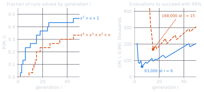
Half or more of the runs failed. Most failures are not near misses of the kind the hits criterion would forgive. In the quadratic runs, seed 3 ended with $x + 1.38$, seed 4 with $x^2 + x + 0.9666$ (error 0.70: the constant is 0.033 too small, more than the 0.01 tolerance), and seed 0 with an 85-node rational function of error 1.38. The script does not measure diversity, but a likely cause is the premature convergence familiar from genetic algorithms: with tournaments of 7 and no mutation, a population that has converged on a wrong structure has few ways to leave it.
Watching one run
The quartic run with seed 11 shows what a run looks like from the inside. The script tools/experiments/evolution/gp_curves.py repeats the runs of the table above and records the best program of every generation. For seed 11:
| Generation | Best program | Size | Error |
|---|---|---|---|
| 0 | (+ (* x x) (sin x)) |
6 | 5.9652 |
| 1 | (* x (exp x)) |
4 | 3.4659 |
| 5 | (+ (sin x) (* x (+ (sin x) (* x (* (sin x) (exp x)))))) |
15 | 0.7429 |
| 16 | (+ (+ (sin (sin x)) (* x x)) (* x (* (sin x) (* x (exp x))))) |
17 | 0.4526 |
| 45 | (+ x (* x (+ x (* x (+ x (* x x)))))) |
13 | 0.0000 |
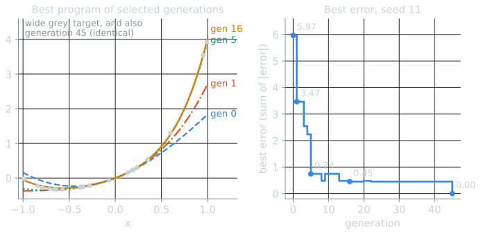
The early programs show how GP uses its vocabulary. None of them is a polynomial, but all of them behave like one near 0, which is where most of the fitness cases lie. Expanding each in a Taylor series about 0 (the script fits the coefficients numerically, rounded to three decimals) shows what each generation has learned:
| Generation | Coefficients of $x$, $x^2$, $x^3$, $x^4$ near 0 |
|---|---|
| target | 1, 1, 1, 1 |
| 0 | 1, 1, −0.167, 0 |
| 1 | 1, 1, 0.5, 0.167 |
| 5 | 1, 1, 0.833, 0.833 |
| 16 | 1, 1, 0.667, 1 |
| 45 | 1, 1, 1, 1 |
From the first generation the best program gets the two lowest-order terms right, since $\sin x \approx x$ and $x e^x \approx x + x^2$; later generations approach the higher coefficients, which matter only for larger $\lvert x \rvert$. The products of $\sin$ and $\exp$ are standing in for powers of $x$. For 29 generations the population could not improve on the generation-16 program, an approximation that is within about 0.02 of the target at a typical fitness case, before one crossover assembled the exact nested form. Plateaus followed by a sudden jump recur in these runs: the quartic run with seed 9 had a best error of 2.2332 from generation 3 to generation 13 and found an exact program at generation 14. A run that has stalled is not necessarily finished.
What the successful programs compute
The evolved trees are rarely the shortest form. To read them, the script evaluates each program at 61 points of $[-2, 2]$, fits polynomials of increasing degree, and reports the polynomial whenever it reproduces the program to within $10^{-6}$ at 401 other points. Some successful quadratic programs:
| Seed | Evolved program | Size | Simplified |
|---|---|---|---|
| 2 | (+ (% x x) (+ x (* x x))) |
9 | $x^2 + x + 1$ |
| 1 | (+ (% x x) (* (+ (% x x) x) x)) |
11 | $x^2 + x + 1$ |
| 22 | (+ (+ (% x x) (- (* x x) (% x -1.236))) (* (% x x) (+ x (% x -1.236)))) |
21 | $x^2 + x + 1$ |
| 11 | (+ (* x x) (- x -0.9929)) |
7 | $x^2 + x + 0.992874$ |
| 9 | 31 nodes with constants $-3.698$, 4.734, 4.012, 1.114 | 31 | $x^2 + x + 1.00795$ |
Nine of the 14 successful programs are exactly $x^2 + x + 1$. Seed 22's contains two terms that cancel. Reading it by hand, with $c = -1.236$ (the constant is $-1.2364563\ldots$, and its value does not matter):
(% x x)is 1 wherever it appears, so the program is(+ (+ 1 (- (* x x) (% x c))) (* 1 (+ x (% x c)))).- The left branch is $1 + (x^2 - x/c)$, and the right branch is $1 \cdot (x + x/c)$.
- Their sum is $1 + x^2 - x/c + x + x/c$, and the two terms in $x/c$ cancel, leaving $x^2 + x + 1$.
The cancellation is exact for every $c \neq 0$, so the evolved constant does no work at all: it is a small piece of code that computes nothing, of the kind the bloat article calls an intron. Seeds 11 and 9 found the right structure with a constant that is slightly off, close enough that every case is a hit; seed 11's error of 0.0071 per case passes the 0.01 tolerance. The remaining three successes, of 45, 65 and 91 nodes, are rational functions that stay within 0.01 of the target at all 21 cases without being equal to it. Their median size, 10 nodes [Q1 9, Q3 28.5], against a minimum of 7, is a first sign of the growth studied in bloat in genetic programming.
The quartic runs show the same range. Seeds 2, 11, 17 and 27 found 13-node trees that simplify exactly to $x^4 + x^3 + x^2 + x$, such as seed 11's nested form (+ x (* x (+ x (* x (+ x (* x x)))))), which is Horner's rule, $x(1 + x(1 + x(1 + x)))$. Seed 9's 27-node program is also exact, but it contains (rlog (exp x)), which is just $x$, and (exp (rlog (- x x))), which is $e^{0} = 1$ because the protected logarithm returns 0 at 0. Such code computes nothing new and is a simple instance of the introns discussed in the bloat article.
Hits are not equality
Seed 28's successful quartic program is
(+ (* x (+ x (exp (rlog (* (+ (* x x) x) x))))) x)
Since $\exp(\mathrm{rlog}(u)) = \lvert u \rvert$ for $u \ne 0$, it computes $x \cdot (x + \lvert x^3 + x^2 \rvert) + x$. For $x > -1$, $x^3 + x^2 = x^2(x + 1)$ is non-negative, the absolute value does nothing, and the program equals the quartic, with error below $10^{-15}$ at every fitness case. For $x < -1$ it does not: at $x = -2$ it returns $-6$ where the quartic gives 10. At $x = -1$ exactly, the protected logarithm of 0 makes the program return $-1$ instead of 0. The smallest fitness case is $-0.991$, so nothing in the data could reveal the difference. Seed 5's program, $e^{x^2} (x + x^2) \cos(x \sin(\sin x))$, is a different kind of near miss: it is an approximation within 0.0052 of the quartic at every case, but at $x = 2$ it returns $-2.41$ instead of 30.
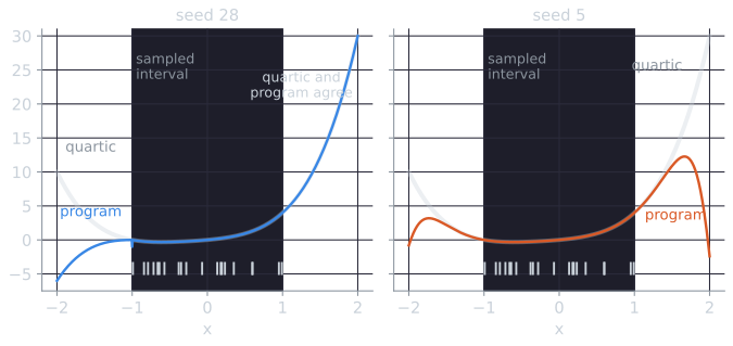
The two programs fail in different ways. Seed 28's program is the quartic over a region that happens to include the data, and differs from it by a sign flip in an absolute value, so it is exactly right or very wrong depending on the side of $-1$. Seed 5's is an approximation everywhere, good where the data are and poor where they are not, which is what any flexible model fitted to data on $[-1, 1]$ tends to be.
Generalization and overfitting
A model found by fitting data has to be judged on data it was not fitted to. For the quartic, the script measures each best-of-run program's mean absolute error against the true function on 401 evenly spaced points, inside the sampled interval and on the wider interval $[-2, 2]$:
| Best-of-run programs | Exact on $[-2, 2]$ | MAE on $[-1, 1]$, median [Q1, Q3] | MAE on $[-2, 2]$, median [Q1, Q3] |
|---|---|---|---|
| 10 successful runs | 5 | 0.0001 [0.0000, 0.0017] | 0.62 [0.00, 1.31] |
| 20 unsuccessful runs | 0 | 0.025 [0.010, 0.041] | 2.50 [1.95, 3.12] |
Inside the sampled interval the successful programs interpolate well. Outside it, only the five exact ones are reliable, and the median error of the successful runs is 0.62 because half of them are approximations. Extrapolation is where an approximation and the true law part company, and it is also where a formula is most useful, since data inside the interval could be interpolated without one.
Overfitting appears when the data contain noise. The script's fourth part draws one data set of 20 points with $x$ uniform on $[-1, 1]$ and $y = x^2 + x + 1$ plus Gaussian noise with standard deviation 0.1. GP runs as before, without the hits criterion, for all 50 generations, and each generation the program with the lowest training error is scored on 401 noise-free points of the target. The true function itself has a training mean absolute error of 0.0723 on this sample, because the noise is in the data; any program with lower training error is fitting the noise.
| Generation | Training MAE | Test MAE | Program size |
|---|---|---|---|
| 0 | 0.2859 [0.2611, 0.3649] | 0.2909 [0.2609, 0.3737] | 7 [5, 14] |
| 5 | 0.0877 [0.0723, 0.1558] | 0.0755 [0.0000, 0.1710] | 11 [9, 15] |
| 10 | 0.0723 [0.0714, 0.0976] | 0.0609 [0.0000, 0.0985] | 16 [9, 21] |
| 20 | 0.0668 [0.0577, 0.0764] | 0.0707 [0.0361, 0.0894] | 54 [14, 70] |
| 30 | 0.0639 [0.0537, 0.0723] | 0.0700 [0.0436, 0.0894] | 74 [30, 104] |
| 40 | 0.0574 [0.0522, 0.0723] | 0.0689 [0.0445, 0.0896] | 95 [24, 120] |
| 50 | 0.0562 [0.0499, 0.0722] | 0.0714 [0.0445, 0.0891] | 100 [38, 129] |
(Medians over 30 runs, with the first and third quartiles in brackets.) In 14 of the 30 runs, the best program of some generation was exactly $x^2 + x + 1$, with test error zero; the zeros in the first quartile at generations 5 and 10 are these runs. Only 4 of the 14 still had it at generation 50. In the others, selection replaced the true law with larger programs that matched the noisy training points more closely. By generation 50, 22 of the 30 final programs had a training error below the true function's 0.0723, and in 22 runs the final test error was more than 10% above the best test error reached earlier in the run. Training error kept falling after generation 10 while test error did not, and program size grew more than sixfold over the same period.
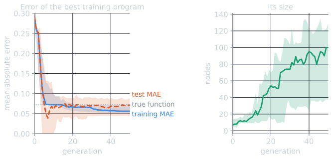
The dotted line is the useful reference. A program can only go below it by matching the particular noise in the 20 training points, which tells nothing about the function. Everything gained below the line in the left panel was paid for with the extra nodes in the right panel.
The remedies are those of any learning method. Data are split into a training set used for fitness and a separate set used to choose among programs and to report results, and a third set is held back when the second has been used for selection. Simpler programs are preferred, which in GP means some form of parsimony pressure on size; this is one motivation for the size-control methods in bloat in genetic programming. Such methods trade some training accuracy for simpler models and are tuned on held-out data.
Modern symbolic regression
Schmidt and Lipson (2009) applied symbolic regression to motion-tracking data from physical systems, from simple harmonic oscillators to chaotic double pendula. A formula that fits the data is not enough to be interesting, so they proposed a criterion for what makes a discovered relation nontrivial. Without prior knowledge of physics, kinematics or geometry, their algorithm found Hamiltonians, Lagrangians and other laws of geometric and momentum conservation. Its demonstrations used systems whose laws were already known, which is what allowed the results to be checked.
Comparisons across methods became more systematic with SRBench (La Cava et al., 2021), an open benchmark of 14 symbolic regression methods and 7 machine learning methods on 252 regression problems. Each method was given a fixed budget, for the real-world problems 500,000 evaluations or 48 hours per training run. The findings include:
- On real-world data sets with no known model, four of the five most accurate methods were GP-based, and the most accurate was Operon, a GP system with nonlinear least-squares optimization of constants. Operon, FEAT and SBP-GP were significantly more accurate than LightGBM, and Operon and SBP-GP more accurate than XGBoost, while the models of the top methods other than SBP-GP were one to three orders of magnitude smaller than those of the tree ensembles.
- On synthetic problems with known equations from physics and dynamical systems, AI Feynman, a physics-inspired method that is not GP-based, recovered the exact equation in 53% of noise-free cases, about twice as often as the next method. At noise levels above 0.01, four other methods recovered exact solutions more often.
- Operon, the most accurate on real-world data, rarely recovered the exact equations of the synthetic problems, despite finding many models with near-perfect test scores.
The last finding repeats, on a larger scale, the distinction between fitting and identifying that seeds 5 and 28 show above. The benchmark's authors also note that the field has relied on small, easy problems and on comparisons with basic GP systems of the kind Koza described. The quartic and the quadratic are such problems: useful for teaching the mechanics, and not evidence of how a method performs on real data.
References
- Keijzer, M. (2003). Improving symbolic regression with interval arithmetic and linear scaling. In C. Ryan et al. (eds.), Genetic Programming: EuroGP 2003, Lecture Notes in Computer Science 2610, 70–82. Springer.
- Koza, J. R. (1992). Genetic Programming: On the Programming of Computers by Means of Natural Selection. MIT Press.
- La Cava, W., Orzechowski, P., Burlacu, B., de França, F. O., Virgolin, M., Jin, Y., Kommenda, M., and Moore, J. H. (2021). Contemporary symbolic regression methods and their relative performance. In Proceedings of the Neural Information Processing Systems Track on Datasets and Benchmarks, vol. 1. arXiv:2107.14351.
- Poli, R., Langdon, W. B., and McPhee, N. F. (2008). A Field Guide to Genetic Programming, chapters 3, 4 and 12. Lulu.com.
- Schmidt, M., and Lipson, H. (2009). Distilling free-form natural laws from experimental data. Science, 324(5923), 81–85.