Thirty runs of genetic programming (GP) on Koza's quartic $x^4 + x^3 + x^2 + x$, with no limit on program size, start from populations whose programs average 13 nodes. Fifty generations later the average is 524 nodes (median over the runs), and the largest program in a typical run has more than 1,800. Ten of the runs found a program that matches the target to within 0.01 at every fitness case, at a median generation of 14. In those ten runs the population's mean size at generation 50 was, at the median, 6.3 times what it had been when the problem was first solved, growth in a population that had nothing left to improve. This growth is bloat.
Bloat is not the same as growth. GP usually starts from small random programs, and a problem may need larger ones; in symbolic regression programs often have to grow to fit all the fitness cases. Poli, Langdon and McPhee (2008, §11.3) therefore define bloat as program growth without (significant) return in terms of fitness. It has practical costs: large programs are expensive to evaluate and to store, hard to read, and they may generalize poorly. This article describes what the extra code consists of, the main explanations of why it accumulates, the methods used to control it, and a seeded comparison of those methods. The experiment uses tools/experiments/evolution/bloat.py in the site repository and the GP system of the symbolic regression article.
Introns
Much of the extra code in a bloated program does nothing. Programs evolved in the symbolic regression runs contain pieces such as these, built from Koza's primitives $\{+, -, \times, \%, \sin, \cos, \exp, \mathrm{rlog}\}$:
| Fragment | Value | Why |
|---|---|---|
(- x x) |
0 | |
(+ y (- x x)) |
$y$ | adds zero |
(* y (% x x)) |
$y$ | protected division makes (% x x) equal 1, even at $x = 0$ |
(exp (rlog (- x x))) |
1 | the protected logarithm returns 0 at 0 |
(rlog (exp x)) |
$x$ | $\log \lvert e^x \rvert = x$ |
By analogy with the stretches of DNA that are removed before a gene is translated, such code is called an intron. Poli, Langdon and McPhee (2008, §11.3.1) use the broader distinction between active code and inactive code: inactive code is code that is not executed, or is executed but its output is then discarded. A subtree such as (- x x) inside (* (- x x) z) is the reverse case: it is active and makes the whole of $z$ inactive, whatever $z$ contains. The distinction can depend on the fitness cases. A subtree whose effect is invisible on every case is inactive as far as selection can tell, even if it would matter for other inputs.
A whole program shows how much of this can accumulate. Seed 9 of the quartic runs in the symbolic regression article found the exact target at generation 14 with a 27-node program:
(+ (+ (+ (rlog (exp x)) (* (* x x) (exp (rlog (- x x))))) (- x x))
   (* (* x x) (+ x (* x x))))
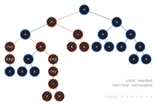
Read from the leaves up, the left half of the tree is $\mathrm{rlog}(e^x) + x^2 \cdot e^{\mathrm{rlog}(0)} + 0 = x + x^2 \cdot 1 + 0$, and the right half is $x^2 (x + x^2) = x^3 + x^4$. Deleting the three detours, 12 nodes in all, leaves the 15-node program (+ (+ x (* x x)) (* (* x x) (+ x (* x x)))) with the same values (the figure script checks this at 41 points). So 44% of this solution, found at generation 14, was code that did nothing. Selection could not see that code: it was carried along inside programs that were selected for what the rest of their code computed.
Introns change what crossover does. A crossover point inside inactive code changes nothing about the program's behavior, so the child has the parent's fitness. As programs fill with inactive code, a growing share of crossovers become neutral.
The uncontrolled runs of the experiment below let this be measured. After every generation, tools/experiments/evolution/gp_curves.py performs 200 extra crossovers between tournament winners of that generation, outside the run, and counts how many children have exactly the same error as their first parent.
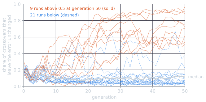
The result is less uniform than the simple story suggests. At generation 0 about a fifth of crossovers are neutral (median 0.198), and about two thirds of those (median 0.120 of all crossovers) return an exact copy of the parent because the two exchanged subtrees were identical. In nine runs the share then climbed past one half, and these are runs in which programs became mostly inactive code: the run with seed 27 found an exact solution and by generation 50 left 97% of crossovers neutral. In the other 21 runs it stayed low, even though their programs were, if anything, larger (median mean size 635 nodes at generation 50, against 400 in the nine). A likely reason, which the script does not test, is that in those runs much of the extra code was active but nearly irrelevant, such as long chains of operations whose effect on the output was small but not zero, so that almost any change to it changed the error a little. Exact neutrality is one way bloat shows itself, not the only one.
Why programs grow
Many explanations of bloat have been proposed, and Poli, Langdon and McPhee (2008, §11.3) note that no single, universally accepted theory explains the full range of observations. The main lines are the following.
Replication accuracy, or protection. McPhee and Miller (1995) showed analytically, for specific cases, that a pressure for accurate replication increases tree size: among fit programs, larger trees are more likely to produce children that compute the same function as their parent. A fit program whose children are as fit as it is has more fit descendants, and inactive code is what makes children faithful. On this view introns spread because they protect good code from destructive crossover.
Removal bias. Soule and Foster (1998) observed that inactive code tends to sit low in the tree, in subtrees smaller than average. A crossover that removes an inactive subtree leaves fitness unchanged, and the subtree inserted in its place is, on average, larger than the one removed. Neutral offspring are therefore larger than their parents on average while keeping their fitness.
The nature of program search spaces. Langdon and Poli (1998) compared runs of the artificial ant problem with and without fitness-based selection, and found that the tendency of solutions to grow is caused by fitness-based selection; their title states the conclusion, "fitness causes bloat". Their argument concerns the space being searched. With a variable-length representation there are many more long programs than short ones for any given fitness, and once fitness stops improving the search mostly finds programs with the same fitness as existing ones. Sampling among those, it finds long ones more often simply because there are more of them. Langdon, Soule, Poli and Foster (1999) developed the account further; Poli, Langdon and McPhee (2008, §11.3.1) summarize it as the prediction that above a certain size the distribution of fitness does not vary with size.
The size evolution equation. These explanations are qualitative. Poli and McPhee (2003) derived from their schema theory an exact equation for the expected mean program size in a GP population, expressed through the selection probabilities of program shapes. Poli and McPhee (2008) later simplified it to the form given by Poli, Langdon and McPhee (2008, §11.3.1):
$$E[\mu(t + 1)] = \sum_{\ell} \ell \, p(\ell, t),$$
where $\mu(t + 1)$ is the mean size of the programs at generation $t + 1$, $\ell$ ranges over program sizes, and $p(\ell, t)$ is the probability that selection picks a program of size $\ell$ from generation $t$. It holds for selection combined with any symmetric subtree crossover, one in which the probability of choosing particular crossover points does not depend on the order in which the parents are drawn. Subtracting the current mean gives
$$E[\mu(t + 1) - \mu(t)] = \sum_{\ell} \ell \, \bigl(p(\ell, t) - \Phi(\ell, t)\bigr),$$
with $\Phi(\ell, t)$ the proportion of programs of size $\ell$ in generation $t$. The equation does not explain bloat by itself, but it constrains every explanation. Crossover alone leaves the expected mean size unchanged: the mean size moves only if selection picks some sizes more often than they occur. For the mean to grow, larger programs must on the whole be selected more often than their share of the population.
The reason is short. A child made by crossover is its first parent with one subtree replaced by a subtree of the second. If both parents are drawn by the same selection and the crossover point in each is chosen by a rule that looks only at that parent, the removed subtree and the inserted subtree have the same expected size, so the child's expected size is that of a selected parent. The experiment below checks this numerically.
A four-program example
The equation can be checked exactly on a population small enough to enumerate. Take four programs over $\{+, \times\}$ and $x$, with errors chosen for the example, and select parents by tournaments of size 2 drawn with replacement. With $N$ programs ranked from best ($r = 1$) to worst, the program of rank $r$ wins a tournament when both entrants are ranked $r$ or worse but not both worse, which has probability $\bigl((N - r + 1)^2 - (N - r)^2\bigr)/N^2$. The numbers below are printed by tools/experiments/evolution/bloat_toy.py:
| Program | Tree | Size $\ell$ | Error | $P(\text{selected})$ |
|---|---|---|---|---|
| A | (+ x (* x x)) |
5 | 1 | 7/16 |
| B | (+ (* x x) (* x (+ x x))) |
9 | 2 | 5/16 |
| C | (* x x) |
3 | 3 | 3/16 |
| D | x |
1 | 4 | 1/16 |
The population's mean size is $\mu(t) = (5 + 9 + 3 + 1)/4 = 4.5$. The size evolution equation predicts
$$E[\mu(t + 1)] = 5 \cdot \tfrac{7}{16} + 9 \cdot \tfrac{5}{16} + 3 \cdot \tfrac{3}{16} + 1 \cdot \tfrac{1}{16} = \tfrac{90}{16} = 5.625.$$
The script then enumerates every possible crossover: each ordered pair of parents with its probability, and each pair of crossover points. It finds the expected child size to be exactly $45/8 = 5.625$, both with crossover points chosen uniformly over the nodes and with Koza's 90/10 rule. If the parents are drawn uniformly instead, without selection, the expected child size is exactly 4.5, the current mean. Crossover moved nothing; selection added 1.125 nodes, because the two best programs, A and B, are also the two largest.
The same enumeration shows what crossover does to the rest of the distribution. Under uniform crossover points, 15.4% of the children are a single node, such as the child of B and D in which the root of B is the crossover point and x is inserted, although the only single-node program, D, is chosen as a parent only 6.25% of the time. These are the small programs that the crossover bias theory, below, says crossover keeps producing and selection keeps discarding.
Crossover bias. Dignum and Poli (2007) built on the equation. Crossover does not change the mean size, but it does change the rest of the size distribution: repeated crossover pushes a population toward a Lagrange distribution of the second kind, in which small programs are much more frequent than long ones, and it creates a high proportion of very small programs, down to single nodes (Poli, Langdon and Dignum, 2007; Poli, Langdon and McPhee, 2008, §11.3.1). In almost every problem of practical interest, very small programs have no chance of solving it, so selection rejects them, which gives programs of above-average size an advantage. Since crossover keeps producing small programs and selection keeps discarding them, the mean size keeps rising. Dignum and Poli (2007) also found that bloat is more marked when the initial population already has the size distribution that crossover prefers (Poli, Langdon and McPhee, 2008, §5.1.2).
These accounts are not exclusive. Protection and removal bias describe what the extra code is and how it is carried; the search-space argument and crossover bias describe why selection ends up favoring larger programs; the size evolution equation states the condition every account must meet.
Controlling bloat
Practitioners had to control bloat long before its causes were understood, and Poli, Langdon and McPhee (2008, §11.3.2) survey the main methods.
Size and depth limits. The simplest control is a hard limit on the depth or size of offspring. In a common implementation, used by Koza (1992), an offspring that exceeds the limit is discarded and a parent is returned instead. This has a side effect: parents that are more likely to produce oversized children are copied more often, so the population fills with programs that sit just under the limit. Depth limits produce bushy, nearly full trees, and size limits produce long, thin ones (Poli, Langdon and McPhee, 2008, §11.3.2). Alternatives are to give an oversized offspring a fitness of zero, or to retry the operation with new crossover points or new parents.
Parsimony pressure. Size can be made part of fitness. Poli, Langdon and McPhee (2008, §11.3.2) write the method, credited to Koza (1992) and to Zhang and Mühlenbein (1995), as $f(x) - c\,\ell(x)$, with $f$ the original fitness, $\ell$ the program's size and $c$ the parsimony coefficient; for an error to be minimized, the equivalent is $e(x) + c\,\ell(x)$. The difficulty is the coefficient. Too small, and runs still bloat; too large, and GP minimizes size at the expense of fitness and converges toward tiny, useless programs. Good values depend on the problem, the primitives and the other parameters. Zhang and Mühlenbein (1995) adjusted the coefficient during the run. Poli and McPhee (2008) derived it from the size evolution equation: their covariant parsimony pressure recomputes $c = \mathrm{Cov}(\ell, f) / \mathrm{Var}(\ell)$ every generation, from the covariance of size and fitness and the variance of size in the population, which holds the mean program size near its initial value, apart from a small drift (Poli, Langdon and McPhee, 2008, §11.3.2). Treating size as a second objective rather than a penalty leads to Pareto-based methods, in which a program survives if no other is at least as small and as fit and strictly better in one of the two (see Pareto dominance); the parsimony penalty is the penalty method of constrained optimization applied to a soft limit on size.
Why $c = \mathrm{Cov}(\ell, f)/\mathrm{Var}(\ell)$ holds the mean size is easiest to see under fitness-proportionate selection, where program $i$ is chosen with probability $f_i / \sum_j f_j$. (The derivation below is ours, for this simplest case.) The size evolution equation then gives
$$E[\mu(t + 1)] = \frac{\sum_i \ell_i f_i}{\sum_i f_i} = \frac{\overline{\ell f}}{\bar{f}} = \mu(t) + \frac{\mathrm{Cov}(\ell, f)}{\bar{f}},$$
using $\overline{\ell f} = \bar{\ell}\bar{f} + \mathrm{Cov}(\ell, f)$, with means and covariance taken over the population. The mean size grows exactly when size and fitness are positively correlated. Replacing $f$ by $f' = f - c\,\ell$ changes the covariance to $\mathrm{Cov}(\ell, f') = \mathrm{Cov}(\ell, f) - c\,\mathrm{Var}(\ell)$, which is zero for the covariant choice of $c$, and then $E[\mu(t + 1)] = \mu(t)$. On the four-program example above, with fitness $f = 5 - \text{error}$, that is 4, 3, 2 and 1 for A to D: $\mathrm{Cov}(\ell, f) = 2.25$ and $\bar{f} = 2.5$, so proportionate selection predicts a mean size of $4.5 + 2.25/2.5 = 5.4$. With $\mathrm{Var}(\ell) = 8.75$, the coefficient is $c = 2.25/8.75 = 0.2571$, the penalized fitnesses are 2.714, 0.686, 1.229 and 0.743, and the predicted mean size is exactly 4.5. The large program B, second best on error, becomes the least likely parent. The penalty is not aimed at any particular program; it cancels, on average, the advantage that size has been getting from its correlation with fitness. Since $c$ is recomputed from each generation's population, the control adapts as that correlation changes.
Lexicographic parsimony pressure. Luke and Panait (2002) avoided the coefficient by using size only to break ties: in a tournament, the fitter program wins, and when two programs are equally fit, the smaller one wins. The method depends only on the ranking of fitness values, not on their scale. In their experiments it reduced tree size while keeping good fitness, particularly when combined with Koza-style depth limits. Its effect depends on how often ties occur, which is often in problems with few distinct fitness values and rarely in regression, where errors are continuous.
The Tarpeian method. Poli (2003) controlled bloat by acting directly on the selection probabilities in the size evolution equation. Each program whose size is above the population average is, with a fixed probability $p$, given the worst possible fitness, which keeps it from becoming a parent. The name comes from the Tarpeian Rock in Rome, from which traitors were thrown. Only the oversized programs are penalized, and only some of them, at random; the others compete normally. Programs that are penalized need not be evaluated, which saves time (Poli, Langdon and McPhee, 2008, §11.3.2). The rate $p$ sets the strength of the control.
Operator equalisation. Dignum and Poli (2008) turned the analysis of size distributions into a control. Operator equalisation controls how GP samples each class of program lengths, which biases the search toward shorter or longer programs or toward specific lengths. The authors describe this as total control over the length distribution, freeing GP from bloat, and they reported that simple length biases could significantly improve the best fitness found for particular classes of problems.
Variation operators. Some operators limit growth themselves. Size-fair crossover chooses the second crossover point so that the inserted subtree is not much larger than the removed one, and hoist and shrink mutation never make a tree larger (Poli, Langdon and McPhee, 2008, §11.3.2; see initialization and variation in genetic programming).
An experiment on the quartic
bloat.py runs Koza's quartic with the GP system and fitness cases of the symbolic regression article: 20 fitness cases on $[-1, 1]$, Koza's function set with terminal $x$, fitness the sum of absolute errors, a population of 500, ramped half-and-half initialization, tournaments of 7, 90% subtree crossover and 10% reproduction. Every run lasts the full 50 generations, so that growth after a solution is found remains visible. Seven conditions are compared, each over seeds 0 to 29; runs with the same seed start from the same initial population.
- No limit: no depth limit and no size control.
- Depth 17: a crossover child deeper than 17 is replaced by a copy of its first parent.
- Parsimony, $c = 0.001$ and $c = 0.01$: tournaments compare error plus $c$ times size, with no depth limit. At $c = 0.01$ a 100-node program pays 1.0, against a typical best error of 3.9 at generation 0.
- Tarpeian, $p = 0.3$ and $p = 0.6$: after the offspring of a generation are created, each one larger than their mean size is, with probability $p$, given infinite error without being evaluated. No depth limit.
- Lexicographic: tournaments compare error, and size only on ties. No depth limit.
Mean program size in the population, median over 30 runs with the first and third quartiles:
| Condition | Gen 0 | Gen 10 | Gen 20 | Gen 30 | Gen 40 | Gen 50 |
|---|---|---|---|---|---|---|
| No limit | 13.3 | 16.3 [11.9, 25.5] | 69.5 [22.5, 90.6] | 200.9 [70.5, 283.7] | 276.5 [130.7, 412.9] | 524.2 [334.4, 771.7] |
| Depth 17 | 13.3 | 16.3 [11.6, 23.5] | 26.4 [19.3, 43.1] | 42.2 [26.1, 53.7] | 44.7 [24.9, 65.8] | 48.0 [28.5, 66.8] |
| Parsimony 0.001 | 13.3 | 14.1 [11.1, 19.5] | 29.5 [19.2, 42.9] | 38.6 [19.2, 61.3] | 42.0 [20.1, 56.7] | 41.0 [19.1, 53.5] |
| Parsimony 0.01 | 13.3 | 12.4 [10.2, 15.4] | 21.2 [15.7, 24.3] | 22.5 [16.2, 26.4] | 23.8 [15.4, 27.9] | 22.1 [15.3, 27.4] |
| Tarpeian 0.3 | 13.3 | 6.6 [6.2, 7.9] | 14.6 [10.6, 19.3] | 16.5 [14.1, 50.3] | 24.6 [13.6, 117.6] | 34.4 [13.6, 226.9] |
| Tarpeian 0.6 | 13.3 | 4.1 [4.0, 4.1] | 4.0 [4.0, 4.1] | 4.1 [4.0, 4.1] | 4.0 [4.0, 4.1] | 4.0 [4.0, 4.1] |
| Lexicographic | 13.3 | 15.5 [11.7, 20.6] | 31.5 [24.1, 53.8] | 62.2 [25.6, 184.7] | 151.1 [22.9, 381.8] | 274.6 [21.4, 861.7] |
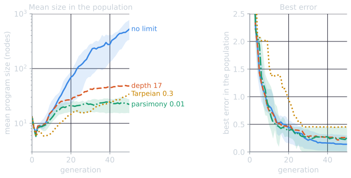
The two panels together are the definition of bloat made visible: in the uncontrolled runs, size rises steeply after generation 10 and keeps rising after generation 30, while the best error falls only slowly, from 0.212 to 0.139 over the last 20 generations.
Best error in the population at generation 50, the number of runs in which some program scored all 20 hits, and the size of the best program at generation 50:
| Condition | Best error, gen 50 | Runs with 20 hits | Best program size, gen 50 |
|---|---|---|---|
| No limit | 0.139 [0.014, 0.297] | 10 | 224 [23, 668] |
| Depth 17 | 0.259 [0.048, 0.427] | 10 | 42 [18, 68] |
| Parsimony 0.001 | 0.272 [0.042, 0.442] | 8 | 43 [15, 75] |
| Parsimony 0.01 | 0.261 [0.006, 0.453] | 12 | 22 [15, 34] |
| Tarpeian 0.3 | 0.451 [0.003, 0.533] | 11 | 24 [13, 178] |
| Tarpeian 0.6 | 3.466 [3.466, 3.466] | 0 | 9 [6, 12] |
| Lexicographic | 0.319 [0.097, 0.453] | 8 | 51 [18, 338] |
The observations, for this problem and these settings:
- Without control, programs bloat. The median mean size grew roughly fortyfold. Best error kept falling slowly, from 0.212 at generation 30 to 0.139 at 50, while mean size grew from 201 to 524. In the ten runs that scored 20 hits, the ratio of the mean size at generation 50 to the mean size when the problem was first solved had a median of 6.3 [2.1, 15.1].
- The depth limit holds the mean size near 48, about a tenth of the uncontrolled size, with the same number of solved runs. The same ratio after solution was 1.21 [1.13, 1.43].
- Parsimony pressure with $c = 0.01$ gave the smallest programs among the conditions that still solved the problem, a best program of 22 nodes at the median, with best errors similar to the depth limit's (median 0.261 against 0.259) and 12 solved runs, the most of any condition. With $c = 0.001$ the penalty was weaker, and sizes were close to those under the depth limit.
- The Tarpeian method's strength matters. With $p = 0.3$ the median run stayed small, but the upper quartile reached a mean size of 227 by generation 50: in a quarter of the runs the control did not stop growth. Its median best error at generation 50, 0.451, was the highest of the conditions that solved the problem at all, although its lower quartile, 0.003, was the lowest. It saved 12.5% of the evaluations. With $p = 0.6$ every run collapsed within ten generations to a population of programs of about four nodes, such as
(* x (exp x)), which has error 3.466, and no run solved the problem. This is the failure that Poli, Langdon and McPhee (2008, §11.3.2) describe for an overly large parsimony coefficient. - Lexicographic parsimony did little here. Its median mean size at generation 50 was 275, about half the uncontrolled size, with a very wide spread [21, 862]. In regression with continuous errors, exact ties are rare, so size is rarely consulted.
Thirty runs per condition on one problem, with one setting for each coefficient, support only modest conclusions. The rankings could change with the problem, the primitives and the coefficients, and none of the published comparisons cited here used this exact system.
Checking the size evolution equation
In the uncontrolled condition every offspring is produced by subtree crossover or reproduction from parents chosen by the same tournament, and crossover points are chosen by Koza's 90/10 rule, which looks only at the parent being cut. The size evolution equation therefore predicts that the expected mean size at generation $t + 1$ equals the mean size of the programs that tournament selection picks at generation $t$. The script estimates $\sum_\ell \ell\, p(\ell, t)$ from 100,000 simulated tournaments on each generation's population and compares it with the mean size actually observed one generation later.
Over all 1,500 pairs of a run and a generation $t = 0, \dots, 49$, the median relative error of the prediction was 1.75%, against a median change in mean size of 9.49% from one generation to the next. For seed 0:
| $t$ | $\mu(t)$ | $\sum_\ell \ell\, p(\ell, t)$ | Observed $\mu(t+1)$ |
|---|---|---|---|
| 10 | 29.0 | 37.7 | 38.1 |
| 20 | 75.8 | 93.0 | 91.5 |
| 30 | 263.1 | 266.8 | 258.7 |
| 40 | 260.6 | 248.4 | 249.2 |
The remaining error is the sampling noise of a single generation of 500 offspring. At generation 10, selection favoured programs 8.7 nodes larger than the population average, and the next generation was larger by almost exactly that amount. At generation 40 it favoured smaller programs, and the mean size fell. Beyond that noise, crossover did not move the mean size; the change came from which programs were selected.
Bloat and generalization
Bloat and overfitting are related but distinct. In the noisy regression experiment of the symbolic regression article, the best programs grew from 16 to 100 nodes between generations 10 and 50 while their training error fell and their error on new data did not. That experiment did not separate the two, but growth of this kind can come from code that fits the noise, which is overfitting, and from inactive code, which is bloat. Size control helps with both by preferring smaller programs, which is why Poli, Langdon and McPhee (2008, §11.3.2) connect parsimony pressure with the trade-off between accuracy and generalization in machine learning. It is not a substitute for testing on held-out data.
References
- Dignum, S., and Poli, R. (2007). Generalisation of the limiting distribution of program sizes in tree-based genetic programming and analysis of its effects on bloat. In Proceedings of the 9th Annual Conference on Genetic and Evolutionary Computation (GECCO 2007), 1588–1595. ACM.
- Dignum, S., and Poli, R. (2008). Operator equalisation and bloat free GP. In M. O'Neill et al. (eds.), Genetic Programming: EuroGP 2008, Lecture Notes in Computer Science 4971, 110–121. Springer.
- Koza, J. R. (1992). Genetic Programming: On the Programming of Computers by Means of Natural Selection. MIT Press.
- Langdon, W. B., and Poli, R. (1998). Fitness causes bloat. In P. K. Chawdhry, R. Roy, and R. K. Pant (eds.), Soft Computing in Engineering Design and Manufacturing, 13–22. Springer.
- Langdon, W. B., Soule, T., Poli, R., and Foster, J. A. (1999). The evolution of size and shape. In L. Spector et al. (eds.), Advances in Genetic Programming 3, ch. 8, 163–190. MIT Press.
- Luke, S., and Panait, L. (2002). Lexicographic parsimony pressure. In GECCO 2002: Proceedings of the Genetic and Evolutionary Computation Conference, 829–836. Morgan Kaufmann.
- McPhee, N. F., and Miller, J. D. (1995). Accurate replication in genetic programming. In L. J. Eshelman (ed.), Proceedings of the Sixth International Conference on Genetic Algorithms, 303–309. Morgan Kaufmann.
- Poli, R. (2003). A simple but theoretically-motivated method to control bloat in genetic programming. In C. Ryan et al. (eds.), Genetic Programming: EuroGP 2003, Lecture Notes in Computer Science 2610, 204–217. Springer.
- Poli, R., Langdon, W. B., and Dignum, S. (2007). On the limiting distribution of program sizes in tree-based genetic programming. In M. Ebner et al. (eds.), Genetic Programming: EuroGP 2007, Lecture Notes in Computer Science 4445, 193–204. Springer.
- Poli, R., Langdon, W. B., and McPhee, N. F. (2008). A Field Guide to Genetic Programming, sections 5.1.2 and 11.3. Lulu.com.
- Poli, R., and McPhee, N. F. (2003). General schema theory for genetic programming with subtree-swapping crossover: Part II. Evolutionary Computation, 11(2), 169–206.
- Poli, R., and McPhee, N. F. (2008). Parsimony pressure made easy. In Proceedings of the 10th Annual Conference on Genetic and Evolutionary Computation (GECCO 2008), 1267–1274. ACM.
- Soule, T., and Foster, J. A. (1998). Removal bias: a new cause of code growth in tree based evolutionary programming. In Proceedings of the 1998 IEEE International Conference on Evolutionary Computation, 781–786. IEEE.
- Zhang, B.-T., and Mühlenbein, H. (1995). Balancing accuracy and parsimony in genetic programming. Evolutionary Computation, 3(1), 17–38.