Suppose a candidate solution can be scored but not solved for. An engineer can simulate the drag of a wing shape but has no formula that returns the best shape. A scheduler can count the clashes in a timetable but cannot write down the clash-free timetable directly. In both cases the only available operation is to propose a candidate and measure how good it is. An evolutionary algorithm (EA) organizes that operation into a loop modeled loosely on natural evolution: keep a population of candidates, let the better ones produce variants of themselves, and let the variants compete with their parents for a place in the next population. Repeated for enough generations, the population tends to move toward better candidates.
This article describes that loop in the general form given by Eiben and Smith (2015, ch. 3), traces one complete run by hand, measures what the loop costs on a problem whose answer is known, and discusses where the method fits. The different families of EA, and how they arose, are the subject of the history of evolutionary computation. The biology behind the metaphor is covered in natural selection for computer scientists.
Three kinds of problem
Eiben and Smith (2015, ch. 1) classify problems by viewing a system as a black box with three parts: an input, a model that transforms it, and an output. A problem arises when one of the three is unknown.
- Optimization. The model is known, and so is the desired output or a measure of how good an output is. The task is to find the input that produces the best output. Designing a wing shape for a known flow simulator, or a timetable for a known set of constraints, is an optimization problem.
- Modelling (system identification). Inputs and their corresponding outputs are known, and the model that connects them is sought. Fitting a formula to measured data, as in symbolic regression, or learning a classifier from labelled examples are modelling problems.
- Simulation. The model and the inputs are known, and the task is to compute the outputs, often to ask what would happen under conditions that have not been observed.
The classification matters because an EA is, at heart, an optimizer. A modelling problem becomes an optimization problem once the candidate models are treated as the inputs and the error on the known examples as the quantity to minimize, which is how genetic programming fits formulas to data. Simulation is different. There an evolutionary process can itself be the model being run, as in studies of artificial life, where the interest lies in what evolves rather than in a single best answer.
The general scheme
Most EAs, whatever their family, follow the same scheme (Eiben and Smith, 2015, ch. 3):
- Initialize a population of candidate solutions, usually at random.
- Evaluate each candidate.
- Repeat until a termination condition holds:
- Select parents from the population.
- Recombine pairs of parents to produce offspring.
- Mutate the offspring.
- Evaluate the offspring.
- Select survivors from parents and offspring to form the next population.
Two forces drive the loop. Variation (recombination and mutation) creates new candidates and so maintains diversity. Selection (of parents and of survivors) favours the better candidates and so pushes quality upward. Neither works alone. Selection without variation can only pick among what already exists, and variation without selection is random search.
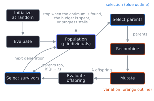
The two kinds of step pull in opposite directions, which is why their balance is the main tuning question in every EA. Selection concentrates the population on what it already does well, and in doing so it removes the differences that variation needs. Variation spreads the population out again, and in doing so it mostly produces candidates that are worse than their parents. The sections below take the parts of the scheme one at a time, and the traced run after them shows how they interact.
Representation
A candidate solution exists at two levels. The phenotype is the solution itself: a wing shape, a timetable, a program. The genotype is its encoding inside the algorithm: a string of bits, a vector of real numbers, a permutation, or a tree. Choosing the representation means choosing the genotype space and the mapping from genotype to phenotype, and it is often the most consequential design decision, because the variation operators act on genotypes. A mutation that changes one bit should usually change the phenotype only a little; when it does not, search becomes erratic. Binary encoding and Gray codes gives a concrete case.
Evaluation function
The evaluation function, or fitness function, assigns each genotype a measure of quality. Together with the representation, it is the channel through which the problem enters the algorithm. In practice it is also where most of the computing time goes, since each evaluation may involve running a simulation or a physical experiment.
Population
The population is a multiset of genotypes: the same genotype may appear more than once. Its size is usually fixed. The population, not the individual, is the unit that changes over time. Individuals are created and discarded; the population persists and its composition shifts. Its diversity, the amount of difference among its members, determines how much the next round of variation has to work with.
Parent selection
Parent selection chooses which individuals reproduce. It is biased toward better individuals but is usually probabilistic, so that weaker individuals keep a small chance of reproducing. That chance matters: an individual that is poor today may carry parts of a better solution, and a selection rule that always picks the best few collapses diversity quickly. Tournament selection, used in the example below, draws $k$ individuals at random and keeps the best of them. How strongly selection favours the best is the subject of selection pressure and premature convergence.
Variation: recombination and mutation
Recombination, or crossover, combines information from two or more parents into one or more offspring. One-point crossover on strings cuts both parents at the same random position and swaps the tails. Recombination can join good parts found separately by different individuals, but crossover of this kind cannot put a value at a position where no parent has it.
Mutation takes one individual and makes a small random change to it. Bit-flip mutation flips each bit independently with a small probability $p_m$, often $1/L$ for strings of length $L$, so that one bit changes on average. Mutation is the source of new values. Both operators are stochastic, and which one does the main work differs between EA families. Crossover and mutation operators covers the standard operators for each representation.
Survivor selection
Survivor selection, or replacement, decides which individuals form the next population. Unlike parent selection, it is often deterministic. Two common rules come from evolution strategies (Beyer and Schwefel, 2002). In $(\mu + \lambda)$ selection, the $\mu$ parents and $\lambda$ offspring are pooled and the best $\mu$ survive, so the best individual found so far is never lost. In $(\mu, \lambda)$ selection, the parents are discarded and the best $\mu$ of the $\lambda$ offspring survive, which lets the population leave a region it has stalled in. The trade-off is examined in $(\mu,\lambda)$ selection and self-adaptation.
Termination
An EA has no natural stopping point, because it cannot in general recognize the optimum. Runs stop when a known optimal fitness is reached, when a budget of evaluations or time is spent, when fitness has not improved for some number of generations, or when diversity has fallen so far that variation produces nothing new.
A run traced by hand
OneMax is the simplest test problem for binary EAs: the genotype is a string of $L$ bits, and the fitness is the number of ones. The optimum, the all-ones string, is known in advance, so the progress of a run is easy to read. Take $L = 8$, a population of $\mu = 4$, and the following settings:
- Parent selection: binary tournament ($k = 2$), drawing with replacement.
- Recombination: one-point crossover on every pair of parents.
- Mutation: bit-flip with $p_m = 1/8$.
- Survivor selection: $(\mu + \lambda)$ with $\lambda = 4$; ties are broken in favour of parents.
Bit positions are numbered 1 to 8 from the left. The run below is produced by the script tools/experiments/evolution/onemax_loop.py in the site repository, with seed 4. The initial population, drawn at random:
| Individual | Genotype | Fitness |
|---|---|---|
| A | 01011000 | 3 |
| B | 01100110 | 4 |
| C | 01001100 | 3 |
| D | 11101100 | 5 |
What the operators will do, on average
Before following the random choices of one run, it helps to compute what the operators do to this population in expectation. Each figure below is exact and comes from the script tools/experiments/evolution/loop_arithmetic.py.
Selection. A binary tournament draws two individuals uniformly with replacement, so there are $4 \times 4 = 16$ equally likely ordered draws, and keeps the fitter one (the first drawn, on a tie). D, the best, wins every draw that contains it. The draws that miss D are the $3 \times 3 = 9$ draws from A, B and C, so D wins with probability $1 - 9/16 = 7/16$. B wins when D is absent and B is present: the 9 draws from A, B and C minus the 4 draws from A and C alone, so $5/16$. A and C split the remaining $4/16$ equally, $1/8$ each. One generation runs four tournaments, two for each of the two crossovers that make the four children, so the expected number of times each individual is chosen as a parent is four times its probability of winning:
| Individual | Fitness | Tournament: P(win); times chosen | Fitness-proportional: $f_i / \sum f$; times chosen |
|---|---|---|---|
| A | 3 | 1/8; 0.50 | 3/15; 0.80 |
| B | 4 | 5/16; 1.25 | 4/15; 1.07 |
| C | 3 | 1/8; 0.50 | 3/15; 0.80 |
| D | 5 | 7/16; 1.75 | 5/15; 1.33 |
The "times chosen" columns are expected values over the four draws of one generation, rounded to two decimals.
The tournament gives the best individual three and a half times as many expected offspring as the worst ones, while the fitness-proportional rule of the classical genetic algorithm gives it only $5/3$ times as many, since it compares fitness values rather than ranks. This ratio is one way of measuring selection pressure. A stronger pressure climbs faster and loses diversity faster, and the trace below shows both.
Mutation. With $p_m = 1/8$ on 8 bits, the number of flipped bits follows a binomial distribution with mean $8 \times 1/8 = 1$. A child is left unchanged with probability $(7/8)^8 = 0.344$, has exactly one bit flipped with probability $8 \cdot (1/8)(7/8)^7 = 0.393$, two with probability 0.196, and three or more with probability 0.067 (rounded to three decimals). So about a third of all children are exact copies of what crossover produced. The same holds for long strings: with $p_m = 1/L$, the probability of no flip is $(1 - 1/L)^L$, which tends to $1/e \approx 0.368$ as $L$ grows (0.364 for $L = 50$).
Crossover. One-point crossover of two parents can only produce something new where the parents differ, and only when the cut separates two such positions. D (11101100) and C (01001100) differ only at positions 1 and 3. A cut after bit 1 or bit 2 separates them; a cut after bit 3 or later, five of the seven possible cuts, returns two exact copies of the parents. Crossover between similar parents is mostly a copying operation, which is why it loses its power as a population converges.
The run
Generation 1. The first tournament draws B and D and picks D (fitness 5); the second draws C and A, a tie at 3, and picks C. One-point crossover cuts after bit 7, one of the five cuts that change nothing for this pair: the children are copies of their parents, 11101100 and 01001100. Mutation leaves the first unchanged and flips bits 7 and 8 of the second, giving 01001111, fitness 5. The next two tournaments pick D and B. Crossover after bit 6 gives 11101110 (D's first six bits, B's last two) and 01100100. Mutation leaves the first alone, at fitness 6, and flips bits 3 and 4 of the second, giving 01010100, fitness 3.
The pool now holds the four parents (3, 4, 3, 5) and four children (5, 5, 6, 3). Keeping the best four gives 11101110 (6), 11101100 (5, parent D), 11101100 (5, D's unchanged copy), and 01001111 (5). Mean fitness has risen from 3.75 to 5.25, and the population already holds two identical genotypes.
Generation 2. Three of the four parents chosen are copies of 11101100, and the first pair crosses one copy with another, which changes nothing. The children score 5, 5, 3 and 5, none better than the current survivors, and $(\mu + \lambda)$ selection keeps the population exactly as it was. A generation can pass with no progress at all.
Generation 3. Mutation flips bit 4 of a copy of 11101100, giving 11111100 (6), and crossover of 11101110 with 01001111 followed by a single flip produces 10101111 (6). The survivors are 11101110, 10101111, 11111100 (all 6) and 11101100 (5).
Generation 4. A tournament picks 11111100 and another picks 10101111. Crossover after bit 5 takes the first five bits of one and the last three of the other: 11111 from 11111100 and 111 from 10101111. The child is 11111111, and mutation leaves it alone. The optimum has been found.
| Generation | Best | Mean | Evaluations so far |
|---|---|---|---|
| 0 | 5 | 3.75 | 4 |
| 1 | 6 | 5.25 | 8 |
| 2 | 6 | 5.25 | 12 |
| 3 | 6 | 5.75 | 16 |
| 4 | 8 | 6.75 | 20 |
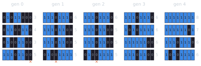
The four tournaments of generation 1 were won by D twice, and by C and B once each, against expected counts of 1.75 for D, 1.25 for B and 0.5 each for A and C. The run then went the way the averages point: D's genes spread through the population, and A's left it.
Each part of the scheme shows up in this short run. Selection let the fitter strings reproduce more often and kept the population from losing ground. Mutation supplied ones that the population lacked: no initial string had a one in position 8 until mutation created one in generation 1, and the one in position 4 of 11111100 also came from mutation, after A, the only initial string with a one there, had been eliminated. Recombination joined two partial solutions, a string that was right in its first five positions and a string that was right in its last three, into one that was right everywhere. The run also shows the loss of diversity that selection causes: by generation 1 the population already contained duplicates, and generation 2 produced nothing usable.
Twenty evaluations is a small fraction of the 256 possible strings. A random search that draws strings uniformly needs 256 draws on average to hit one particular string, since each draw succeeds with probability $1/256$. One lucky run proves nothing, however, and the next section measures the loop properly.
What the loop costs
The same script runs four methods on OneMax with $L = 50$, thirty times each with seeds 1000 to 1029, and records the number of evaluations needed to reach the all-ones string, with a budget of 100,000 evaluations:
- Random search draws strings uniformly.
- The $(1+1)$ EA keeps a single string, mutates it with $p_m = 1/L$, and keeps the child if it is at least as good.
- A population EA uses the scheme of the hand-traced run with $\mu = \lambda = 20$.
- A bit-by-bit method flips each position once, in order, and keeps the flip if fitness rises.
| Method | Runs solved | Evaluations, median | Interquartile range |
|---|---|---|---|
| Random search | 0 of 30 | (best fitness 40 of 50) | (best 39 to 41) |
| $(1+1)$ EA | 30 of 30 | 411 | 385 to 501 |
| Population EA | 30 of 30 | 650 | 600 to 700 |
| Bit-by-bit | 30 of 30 | 51 | 51 to 51 |
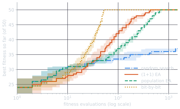
The curves show where each method spends its evaluations. A random string has about 25 ones, with a standard deviation of $\sqrt{50 \cdot \tfrac14} \approx 3.5$, and the best of $m$ independent strings creeps up only slowly with $m$: the median best was 31 after 20 draws, 36 after 1,000 and 37 after 1,500. The $(1+1)$ EA reached a median of 42 after 100 evaluations, 47 after 200 and 49 after 400. Its last few ones cost the most, because once only $i$ zeros remain, an improving mutation must flip one of those $i$ positions without flipping a one elsewhere, which happens with probability at least $i/(eL)$ per evaluation; the fitness landscapes article turns this bound into the $e L \ln L$ estimate of the run time. The population EA follows the same shape, shifted to the right: it evaluates 20 children per generation, and early on most of them duplicate progress another child has already made.
Random search never comes close: the chance that a random 50-bit string is all ones is $2^{-50}$, and after 100,000 draws the best string found typically has 40 ones. Both evolutionary methods solve every run in a few hundred evaluations. Their cost has been analysed exactly: Droste, Jansen, and Wegener (2002) proved that the $(1+1)$ EA needs $\Theta(L \log L)$ evaluations in expectation on OneMax, and on every linear function of the bits. The logarithmic factor comes from the end of the run, when only a few zeros remain and a random mutation rarely hits one of them.
Two results in the table are warnings. First, the population EA, with its crossover and its twenty individuals, needed more evaluations than the single-string $(1+1)$ EA. A population costs evaluations every generation, and on a problem this simple the extra exploration it buys is not needed. Second, the bit-by-bit method needed exactly $L + 1 = 51$ evaluations every time, about an eighth of the EA's cost. It exploits a fact that the EA ignores: in OneMax every bit contributes to fitness independently of every other. When a problem has structure of that kind, a method designed to use it will beat a general-purpose search.
Where an EA is the right tool
The scheme above asks very little of the problem: a representation that variation operators can act on, and an evaluation function. Nothing in it uses derivatives, convexity, or a closed-form model. That makes EAs suited to problems where those are unavailable:
- Black-box evaluation. The quality of a candidate is known only by computing it, through a simulation, a physical experiment, or a game played against an opponent. The first evolution strategies optimized physical shapes in air flow this way (Beyer and Schwefel, 2002).
- Many local optima. A method that only moves uphill from one point, such as hill climbing, stops at the first peak it reaches, as K-means stops at a local minimum of its objective. A population spread over the search space, together with recombination, can reach regions a single trajectory would not. Fitness landscapes makes this picture precise and shows its limits.
- Structured or mixed search spaces. Programs, neural network topologies, schedules and circuit layouts have no natural gradient. Representations and operators can be designed for them, as in genetic programming and neuroevolution.
- Several objectives at once. A population can hold many trade-offs between conflicting goals in a single run, which is the basis of multi-objective evolutionary algorithms.
- Noisy or changing evaluations. Because selection compares many individuals over many generations, the occasional mismeasured fitness does not derail a run.
Where it is not
The same generality is the method's weakness. An EA does not use what is known about a problem unless that knowledge is built into its representation and operators, and several situations call for something else:
- An efficient exact algorithm exists. Shortest paths, minimum spanning trees, sorting and linear programs have algorithms that are both faster and guaranteed correct.
- The objective is smooth and its gradient is cheap. Gradient-based methods use far more information per evaluation, which is why neural networks are usually trained by backpropagation rather than evolved.
- Evaluations are very expensive. A typical EA run uses thousands of evaluations or more. When each one takes hours, methods designed to make the most of a few evaluations, such as surrogate-model and Bayesian optimization, are usually a better start.
- A guarantee is required. An EA does not certify that its answer is optimal, or even how far from optimal it is. Its results are also random: a single run is an anecdote, and a fair comparison needs many seeded runs, as in the table above.
- The structure is known and exploitable. The bit-by-bit result above is the general case in miniature.
Behind these cautions lies a formal result. Wolpert and Macready (1997) proved that, averaged over all possible objective functions, every search algorithm performs equally well. An EA can only outperform random search, or any other method, on a class of problems whose structure suits it. The no free lunch theorems article states the results and what they do and do not imply.
References
- Beyer, H.-G., and Schwefel, H.-P. (2002). Evolution strategies: A comprehensive introduction. Natural Computing, 1(1), 3–52.
- Droste, S., Jansen, T., and Wegener, I. (2002). On the analysis of the (1+1) evolutionary algorithm. Theoretical Computer Science, 276(1–2), 51–81.
- Eiben, A. E., and Smith, J. E. (2015). Introduction to Evolutionary Computing, 2nd ed., chapters 1 and 3. Springer.
- Wolpert, D. H., and Macready, W. G. (1997). No free lunch theorems for optimization. IEEE Transactions on Evolutionary Computation, 1(1), 67–82.