Suppose a population of 100 candidate solutions contains one individual better than all the others, and the algorithm does nothing but select: no crossover, no mutation, each generation formed by choosing 100 individuals from the current one. Copies of the best individual multiply until they fill the population. Under binary tournament selection this takes about 9 generations; under fitness-proportional selection with the same population it can take several hundred, or never happen at all, because the best individual is lost by chance. That speed is one way to measure selection pressure, the degree to which a selection scheme favours better individuals.
Selection pressure is a trade-off. Too little, and the search drifts: good individuals reproduce barely more than poor ones, and the algorithm behaves like random sampling. Too much, and the population fills with copies of whatever was best early on, before crossover and mutation have had time to find anything better. The second failure is premature convergence: the population loses its diversity while it is still far from the optimum, and with no diversity left, recombination has nothing to combine. This article describes the standard selection schemes of a genetic algorithm, two ways to quantify their pressure, and the methods used to keep a population diverse. Eiben and Smith (2015, ch. 5) cover the same material at textbook level.
Fitness-proportional selection
Holland's (1975) original reproductive plan selects each individual with probability proportional to its fitness. With fitness values $f_1, \dots, f_n$, all positive and to be maximized, individual $i$ is chosen with probability
$$p_i = \frac{f_i}{\sum_{j=1}^{n} f_j},$$
and in $n$ selections it receives on average $n p_i = f_i / \bar{f}$ copies, its fitness divided by the population mean $\bar{f}$. The usual picture is a roulette wheel with one slot per individual, each slot's width proportional to fitness.
The scheme depends on the absolute values of fitness, not only their order, and that causes two problems. Take four individuals with fitness 1, 2, 3 and 4. Their expected copies are 0.4, 0.8, 1.2 and 1.6. Add 100 to every value, a change that leaves the ranking and the optimum untouched, and the expected copies become 0.985, 0.995, 1.005 and 1.015. Selection has almost vanished. The same thing happens during a run: early on, a single individual far above the mean can take most of the wheel and fill the population within a few generations, while late in a run, when fitness values cluster closely, the wheel becomes nearly uniform and selection stops pushing. The second effect undermined the course's binary GA on De Jong's test functions, as that article measures.
A short calculation shows why. Let $\sigma$ be the standard deviation of fitness in the population (with divisor $n$, so $\sigma^2 = \frac{1}{n}\sum_i f_i^2 - \bar{f}^2$). The mean fitness of a selected parent is the average of the $f_i$ weighted by their selection probabilities:
$$\bar{f}_{\text{sel}} = \sum_{i=1}^{n} p_i f_i = \frac{\sum_i f_i^2}{\sum_i f_i}.$$
Both sums can be written in terms of the population's mean and variance. The denominator is $\sum_i f_i = n \bar{f}$. Rearranging the definition of $\sigma^2$ gives the numerator, $\sum_i f_i^2 = n(\sigma^2 + \bar{f}^2)$. Dividing,
$$\bar{f}_{\text{sel}} = \frac{n(\sigma^2 + \bar{f}^2)}{n \bar{f}} = \bar{f} + \frac{\sigma^2}{\bar{f}}.$$
The gain from selection, $\bar{f}_{\text{sel}} - \bar{f} = \sigma^2 / \bar{f}$, measured in units of $\sigma$, is therefore $\sigma/\bar{f}$, the coefficient of variation. For the values 1 to 4, $\bar{f} = 2.5$ and $\sigma = 1.118$, so the mean after selection is $30/10 = 3.0 = 2.5 + 1.25/2.5$ and the standardized gain is $1.118/2.5 = 0.447$. For 101 to 104, $\sigma$ is the same but $\bar{f} = 102.5$, so the mean after selection is 102.512 and the standardized gain is 0.011. Adding a constant to fitness leaves $\sigma$ unchanged and inflates $\bar{f}$, and the selection differential shrinks in proportion.
Scaling repairs this by transforming fitness before selection. Windowing subtracts the worst fitness of the current or a recent generation. Sigma scaling uses $f' = \max(f - (\bar{f} - c\,\sigma), 0)$ with a constant $c$, often 2, which makes selection depend only on how many standard deviations an individual lies above the mean (Goldberg, 1989; Eiben and Smith, 2015, ch. 5). On the values 1 to 4 with $c = 2$, the baseline is $\bar{f} - 2\sigma = 2.5 - 2.236 = 0.264$, the scaled values are 0.736, 1.736, 2.736 and 3.736, with sum 8.944, and the expected copies are $4 \times 0.736/8.944 = 0.33$, then 0.78, 1.22 and 1.67. On 101 to 104 the baseline is $102.5 - 2.236 = 100.264$, the scaled values are the same four numbers, and so are the expected copies.
Sampling: roulette wheel and stochastic universal sampling
Selection probabilities say how many copies each individual should receive on average; a sampling algorithm turns them into actual counts. Spinning the wheel $n$ times independently gives each individual a binomially distributed number of copies, so an individual expected to receive 1.6 copies receives none with probability $(1 - 0.4)^4 \approx 0.13$ in a population of four. Baker (1987) analyzed this sampling error and proposed stochastic universal sampling (SUS): a single spin of a wheel with $n$ equally spaced pointers. Every individual then receives either the floor or the ceiling of its expected number of copies, and the expected count is still exact. SUS can be used with any scheme that assigns selection probabilities, including the ranking schemes below.
The difference shows on the four-string population of the simple genetic algorithm article, Goldberg's $x^2$ example, whose strings expect 0.578, 1.969, 0.219 and 1.234 copies. Lay these expectations end to end on a line from 0 to 4. Independent spins drop four points at random on the line. SUS draws one offset $u$ uniformly from $[0, 1)$ and places pointers at $u$, $u + 1$, $u + 2$ and $u + 3$.
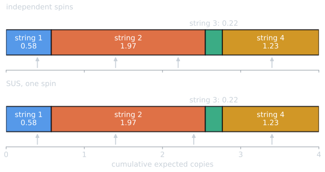
Since the pointers are one unit apart, an interval of width $e$ contains either $\lfloor e \rfloor$ or $\lfloor e \rfloor + 1$ of them, the second with probability $e - \lfloor e \rfloor$. The distributions of the number of copies under the two samplers are then:
| String | Expected | Independent spins, P(0 to 4 copies) | SUS |
|---|---|---|---|
| 1: 01101 | 0.578 | 0.536, 0.362, 0.092, 0.010, 0.000 | P(0) = 0.422, P(1) = 0.578 |
| 2: 11000 | 1.969 | 0.066, 0.258, 0.375, 0.242, 0.059 | P(1) = 0.031, P(2) = 0.969 |
| 3: 01000 | 0.219 | 0.799, 0.185, 0.016, 0.001, 0.000 | P(0) = 0.781, P(1) = 0.219 |
| 4: 10011 | 1.234 | 0.229, 0.408, 0.273, 0.081, 0.009 | P(1) = 0.766, P(2) = 0.234 |
(Probabilities are rounded to three places.) Under independent spins the best string is lost with probability 0.066; under SUS it is never lost and receives two copies 97 percent of the time. Both samplers give the same expected counts, so both implement the same selection scheme. They differ only in the noise around those counts, and that noise is what the takeover experiment below shows to matter.
Rank-based selection
Ranking removes the dependence on fitness values altogether. Individuals are sorted, and selection probabilities are assigned by rank. In linear ranking (Baker, 1985), with ranks $r = 0$ for the worst through $r = n - 1$ for the best and a parameter $s$ with $1 < s \le 2$,
$$p(r) = \frac{2 - s}{n} + \frac{2 r (s - 1)}{n (n - 1)}$$
(Eiben and Smith, 2015, ch. 5). The best individual expects $s$ copies and the worst $2 - s$; $s$ sets the pressure directly. With four individuals and $s = 1.5$ the expected copies are 0.5, 0.833, 1.167 and 1.5, whatever the fitness values are, so adding 100 to every fitness changes nothing. The cost is a sort, $O(n \log n)$ per generation, and the loss of information about how much better one individual is than another.
Tournament selection
Tournament selection draws $k$ individuals at random and selects the best of them, repeating until enough parents are chosen. Goldberg and Deb (1991) trace it to unpublished work by Wetzel studied in Brindle's dissertation. It needs no global sort and no knowledge of the population's fitness distribution, only pairwise comparisons, which makes it easy to parallelize and usable when fitness is defined only by comparison. The tournament size $k$ controls pressure: the best individual in a large population wins a tournament whenever it is drawn, so with replacement it expects about $k$ copies. With four individuals and $k = 2$, the expected copies by rank are exactly 0.25, 0.75, 1.25 and 1.75, since the individual of rank $i$ (counting from 1 for the worst) wins when it is the better of the two drawn, with probability $(i^2 - (i-1)^2)/16$.
Goldberg and Deb (1991) showed that, under their model, in which a population is divided into classes of equal fitness, binary tournament and linear ranking with $s = 2$ are identical in expectation. They also analyzed a probabilistic binary tournament in which the better individual wins only with probability $p$; it matches ranking with $s = 2p$, so every linear ranking scheme has a tournament with the same expected effect. (In a finite population of distinct individuals the two differ slightly, and agree as $n$ grows.)
Truncation selection
Truncation selection keeps the best fraction $T$ of the population and selects uniformly among them; everything below the threshold is discarded. It is the selection of animal and plant breeding, and Mühlenbein and Schlierkamp-Voosen (1993) built their breeder genetic algorithm on it. The survivor selection of evolution strategies, keeping the best $\mu$ of $\lambda$ offspring, is truncation of the same kind (see $(\mu,\lambda)$ selection and self-adaptation).
The schemes side by side
The four-individual example used above makes the schemes easy to compare by hand. The table gives the expected number of copies of each individual, worst to best, when the fitness values are 1, 2, 3 and 4, and when they are 101, 102, 103 and 104. Tournaments draw their contestants with replacement. Values are rounded to three places, except the tournament with $k = 3$, whose values are exact.
| Scheme | Fitness 1, 2, 3, 4 | Fitness 101 to 104 |
|---|---|---|
| Fitness-proportional | 0.400, 0.800, 1.200, 1.600 | 0.985, 0.995, 1.005, 1.015 |
| Sigma scaling, $c = 2$ | 0.329, 0.776, 1.224, 1.671 | the same |
| Linear ranking, $s = 1.5$ | 0.500, 0.833, 1.167, 1.500 | the same |
| Linear ranking, $s = 2$ | 0.000, 0.667, 1.333, 2.000 | the same |
| Tournament, $k = 2$ | 0.250, 0.750, 1.250, 1.750 | the same |
| Tournament, $k = 3$ | 0.0625, 0.4375, 1.1875, 2.3125 | the same |
| Truncation, $T = 0.5$ | 0, 0, 2, 2 | the same |
Only fitness-proportional selection changes between the two columns. Every other scheme depends on the order of the fitness values, or, for sigma scaling, on their distances measured in standard deviations, and both are unchanged by adding a constant. The tournament entries follow from counting: with $k$ contestants drawn with replacement, the individual of rank $i$ (1 for the worst) wins when every contestant has rank at most $i$ and not every contestant has rank at most $i - 1$, which has probability $(i/n)^k - ((i-1)/n)^k$. For $k = 3$ and the best of four, that is $1 - (3/4)^3 = 0.578$, or 2.3125 expected copies.
In a larger population the same comparison becomes a curve. The figure plots expected copies against rank in a population of 100 with one individual in each fitness class $i/100$, the setting of the takeover experiment below.
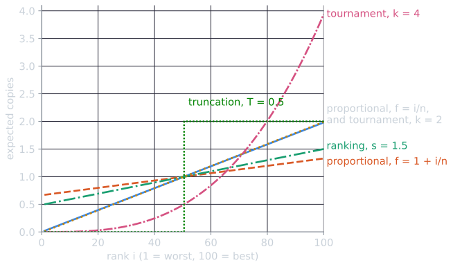
The coincidence of the two top lines is not general. Proportional selection behaves like binary tournament here only because fitness happens to be proportional to rank and to start near zero; shift the fitness values, as the dashed line shows, and the match is gone.
Takeover time
Goldberg and Deb (1991) compared selection schemes by the takeover time $t^*$: the number of generations selection alone needs to grow a single best individual until it occupies $n - 1$ places in a population of $n$. They wrote difference equations for the expected proportion $P_t$ of the best class. For a tournament of size $k$, an individual outside the best class is selected only if all $k$ contestants come from outside it, so $1 - P_{t+1} = (1 - P_t)^k$. For linear ranking with parameter $c_0$ (the expected copies of the best individual, which is $s$ above), $P_{t+1} = P_t \left[ c_0 - (c_0 - 1) P_t \right]$. Solving from $P_0 = 1/n$ to $(n-1)/n$ gives the approximations in their Table 2:
| Scheme | Takeover time $t^*$ |
|---|---|
| Fitness-proportional, $f(x) = x^c$ | $\frac{1}{c}(n \ln n - 1)$ |
| Fitness-proportional, $f(x) = e^{cx}$ | $\frac{1}{c}\, n \ln n$ |
| Linear ranking, $c_0 = 2$ | $\log_2 n + \log_2 (\ln n)$ |
| Linear ranking, $1 < c_0 < 2$ | $\frac{2}{c_0 - 1} \ln (n - 1)$ |
| Tournament of size $k$ | $\frac{1}{\ln k} \left[ \ln n + \ln (\ln n) \right]$ |
The fitness-proportional results assume $n$ individuals spread evenly over the unit interval, with the best at $x = 1$. The ranking formula for $c_0 < 2$ comes from a logistic differential-equation approximation; Goldberg and Deb give it with the natural logarithm and note that base 2 corrects the approximation's early overshoot but overestimates the late phase. The contrast in orders of growth is the main result: ranking and tournament selection take over in $O(\log n)$ generations, fitness-proportional selection in $O(n \log n)$. Goldberg and Deb add a caution. A real GA must assemble good solutions from parts while selection is acting, so takeover time does not predict how fast a GA finds the optimum. It gives an idea of how long a GA can run before mutation becomes its main means of exploration.
Deriving the tournament formula
The tournament entry in the table can be derived in a few lines, and the derivation shows where the $\ln \ln n$ term comes from. Write $Q_t = 1 - P_t$ for the proportion of the population outside the best class.
- One generation. A tournament selects an individual outside the best class only if all $k$ contestants come from outside it. Contestants are drawn independently, so in expectation $Q_{t+1} = Q_t^k$.
- Unrolling. Applying the recursion $t$ times multiplies the exponents: $Q_t = Q_0^{k^t}$, with $Q_0 = 1 - 1/n$. The outside share shrinks doubly exponentially.
- The stopping condition. Takeover means $P_t = (n-1)/n$, that is $Q_t = 1/n$. Taking logarithms of $Q_0^{k^t} = 1/n$ gives $k^t \ln(1 - 1/n) = -\ln n$.
- Approximating. For large $n$, $\ln(1 - 1/n) \approx -1/n$ (for $n = 100$ the two are 0.01005 and 0.01000). Then $k^t / n \approx \ln n$, so $k^t \approx n \ln n$.
- Solving for $t$. Taking logarithms once more, $t \ln k \approx \ln n + \ln \ln n$, which is Goldberg and Deb's formula, $t^* \approx (\ln n + \ln \ln n)/\ln k$.
For $n = 100$ and $k = 2$, the exact solution of step 3 is $t = 8.840$ and the approximation gives 8.847. Following the recursion one generation at a time shows the shape of takeover: the best class's proportion $P_t$ is 0.010, 0.020, 0.039, 0.077, 0.149, 0.275, 0.474, 0.724, 0.924 and 0.994 for $t = 0, \dots, 9$ (rounded to three places). It roughly doubles each generation while it is small, since $1 - (1 - P)^2 \approx 2P$, and then closes the remaining gap in two or three generations, the logistic shape common to all the schemes.
Takeover time measured
The script tools/experiments/evolution/takeover.py in the site repository runs the Goldberg and Deb setting: $n$ individuals, one in each fitness class $f = i/n$ for $i = 1, \dots, n$, selection only, with replacement, for 30 seeds per scheme. Each run stops when the best class holds $n - 1$ places, or when it dies out. The table gives the closed form above, the first generation at which the deterministic recursion reaches $(n-1)/n$, the median and interquartile range of the simulated takeover times over the runs in which the best survived, and the number of runs in which it was lost.
| Scheme, $n = 100$ | Closed form | Recursion | Simulated median [Q1, Q3] | Best lost |
|---|---|---|---|---|
| Proportional, independent spins | 459.5 | 459 | 100.0 [57.0, 117.0] | 17 of 30 |
| Proportional, SUS | 459.5 | 459 | 397.5 [348.5, 486.2] | 0 of 30 |
| Linear ranking, $s = 2$ | 8.8 | 9 | 9.0 [8.5, 10.0] | 7 of 30 |
| Linear ranking, $s = 1.5$ | 18.4 | 19 | 16.5 [15.0, 18.2] | 14 of 30 |
| Tournament, $k = 2$ | 8.8 | 9 | 9.0 [9.0, 10.0] | 5 of 30 |
| Tournament, $k = 4$ | 4.4 | 5 | 5.0 [5.0, 5.0] | 1 of 30 |
| Tournament, $k = 8$ | 2.9 | 3 | 3.0 [3.0, 3.8] | 0 of 30 |
| Truncation, $T = 0.5$ | 7 | 7.0 [6.0, 8.0] | 6 of 30 |
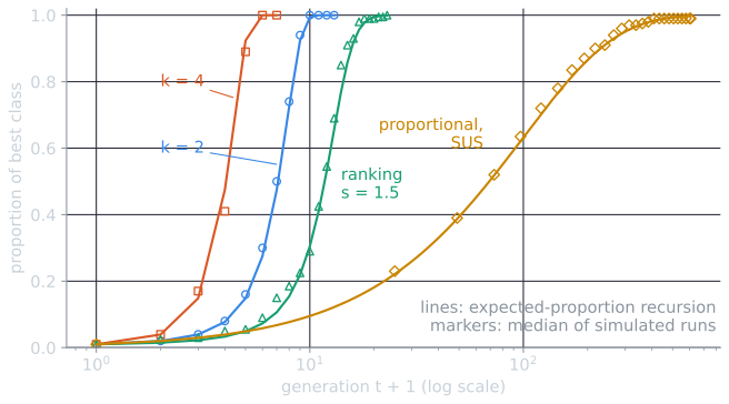
For ranking and tournament selection, the medians agree with the theory to within a generation or two. With $n = 1000$ they grow only slightly, as $O(\log n)$ predicts: 13 generations for binary tournament (theory 12.8) and 5 for $k = 8$ (theory 4.3).
Fitness-proportional selection with independent spins departs from the theory completely. The best individual was lost in 17 of 30 runs, and in the other 13 it took over in a median of 100 generations, not 459. Both effects come from sampling error. The best individual starts with an expected 1.98 copies, and the number it actually receives is close to a Poisson count with that mean, which is zero about 14% of the time. Later, the top classes have nearly equal fitness, the wheel barely distinguishes them, and their numbers wander at random, a process population geneticists call genetic drift. Drift, not selection, then decides which class fills the population, and it does so faster than selection would. With SUS, which removes most of the sampling error, no run lost the best individual and the median of 397.5 generations came much closer to the prediction. At $n = 1000$ the gap is larger still: 544 generations with independent spins, with the best lost in 21 runs, against 6,484 with SUS and a prediction of 6,907.
The column of losses is a result in its own right. Even binary tournament selection, the most common scheme in practice, lost the best individual in 5 of 30 runs, because an individual that is never drawn into a tournament is never copied, which happens to any given individual with probability $(1 - 1/100)^{200} \approx 0.13$. Truncation selection, which never discards the best individual from the candidate pool, still lost it in 6 runs: 100 uniform draws from the top 50 miss a given individual with probability $(1 - 1/50)^{100} \approx 0.13$.
Selection intensity
Takeover time looks at the best individual only. Blickle and Thiele (1996) characterized a scheme by its effect on the whole fitness distribution, borrowing selection intensity from quantitative genetics: the change in mean fitness caused by selection, divided by the standard deviation of fitness before selection,
$$I = \frac{\bar{f}_{\text{sel}} - \bar{f}}{\sigma}.$$
For comparison, they computed $I$ on a population whose fitness follows the standard normal distribution. For a tournament of size $k$, $I$ is the expected maximum of $k$ standard normal values, $1/\sqrt{\pi} \approx 0.5642$ for $k = 2$. For linear ranking, $I = (s - 1)/\sqrt{\pi}$, so ranking with $s = 2$ and binary tournament have the same intensity. For truncation with threshold $T$, $I = \varphi(z)/T$, where $z$ is the point above which a fraction $T$ of the standard normal lies and $\varphi$ is the standard normal density. Fitness-proportional selection is not invariant to translation, so it has no standardized value; the calculation above gives $\sigma/\bar{f}$ for it.
The binary tournament value can be checked by hand. For two numbers, $\max(X_1, X_2) = \frac{1}{2}(X_1 + X_2) + \frac{1}{2}|X_1 - X_2|$. If $X_1$ and $X_2$ are independent standard normal values, the first term has expectation 0. The difference $X_1 - X_2$ is normal with mean 0 and variance 2, and the mean absolute value of a normal variable with standard deviation $s$ is $s\sqrt{2/\pi}$, so $\mathbb{E}|X_1 - X_2| = \sqrt{2} \cdot \sqrt{2/\pi} = 2/\sqrt{\pi}$. Halving it gives $I = 1/\sqrt{\pi} = 0.5642$. The same value for linear ranking with $s = 2$ is no coincidence: Goldberg and Deb's equivalence of the two schemes in expectation, described above, carries over to their effect on a normal population.
Blickle and Thiele also defined the loss of diversity $p_d$, the fraction of the population not selected. Their formulas give the smallest loss the expected numbers of copies allow: summed over the individuals expected to receive fewer than one copy, the shortfall of each one's expectation below one, as a fraction of the population. This gives $p_d = k^{-1/(k-1)} - k^{-k/(k-1)}$ for tournaments, $(s - 1)/4$ for linear ranking, and $1 - T$ for truncation.
The second part of takeover.py checks these on 10,000 standard normal fitness values, 30 seeds, with independent draws:
| Scheme | $I$, theory | $I$, measured | $p_d$, theory | $p_d$, measured |
|---|---|---|---|---|
| Tournament, $k = 2$ | 0.5642 | 0.5641 | 0.2500 | 0.4322 |
| Tournament, $k = 4$ | 1.0294 | 1.0287 | 0.4725 | 0.5613 |
| Tournament, $k = 8$ | 1.4236 | 1.4236 | 0.6501 | 0.6948 |
| Linear ranking, $s = 2$ | 0.5642 | 0.5665 | 0.2500 | 0.4334 |
| Linear ranking, $s = 1.5$ | 0.2821 | 0.2849 | 0.1250 | 0.3840 |
| Truncation, $T = 0.5$ | 0.7979 | 0.7988 | 0.5000 | 0.5675 |
Intensity matches the theory to two or three decimal places. The measured loss of diversity is much larger, because independent draws miss individuals that would have been selected on average. Binary tournament leaves out 43% of the population each generation, not 25%. Ranking with $s = 1.5$, the gentlest scheme in the table, loses 38% under independent sampling and exactly 12.5% under SUS, which the script also prints. How a scheme is sampled can matter as much as which scheme it is.
Elitism
The losses in the takeover experiment have a simple remedy. Elitism copies the best individual, or the best few, into the next generation unchanged. De Jong (1975) studied this as the elitist strategy. It guarantees that the best fitness in the population never decreases, and it has a theoretical justification: Rudolph (1994) proved with a Markov chain model that the canonical genetic algorithm, with proportional selection, crossover and mutation, does not converge to the global optimum in the sense that the probability of the population containing it tends to one, while variants that always keep the best solution do. Plus-selection in evolution strategies, which pools parents and offspring before choosing survivors, is elitist by construction. Elitism also adds pressure, since the elite are never lost and keep reproducing, so it is usually limited to one or a few individuals.
Diversity loss and premature convergence
Premature convergence happens when the population becomes concentrated in one region before any member has found a good solution there. Strong selection is the main cause, but not the only one. Drift, as the experiment shows, can fix an arbitrary class in a finite population without any selective reason, and small populations drift fast. Crossover between near-identical parents produces near-identical children, so once diversity is gone, only mutation can introduce anything new, and at low mutation rates the search becomes a slow local search around one point. De Jong (1975) observed this stall in his own experiments, as the article on the De Jong functions describes.
The remedies follow from the causes: lower selection pressure (smaller tournaments, gentler ranking), sampling with SUS, larger populations, higher mutation rates, restarts when diversity falls below a threshold, and separate subpopulations that exchange individuals only occasionally, as in island models. A different family of methods changes selection itself so that the population keeps several groups, or niches, around different optima.
Niching
On a function with several optima of equal height, a plain genetic algorithm ends up on one of them, chosen largely by drift. Niching methods aim to keep subpopulations on several peaks at once, which helps both when several good solutions are wanted and when the global optimum lies on a peak that would otherwise be abandoned early.
Fitness sharing
Goldberg and Richardson (1987) proposed fitness sharing: individuals close to each other share their fitness, like animals sharing the food of one habitat. Each individual's fitness is divided by a niche count,
$$f'_i = \frac{f_i}{\sum_{j=1}^{n} \mathrm{sh}(d_{ij})}, \qquad \mathrm{sh}(d) = \begin{cases} 1 - (d/\sigma_{\text{share}})^{\alpha} & d < \sigma_{\text{share}}, \\ 0 & \text{otherwise,} \end{cases}$$
where $d_{ij}$ is the distance between individuals $i$ and $j$ (in genotype or phenotype space), $\sigma_{\text{share}}$ is the niche radius, and $\alpha$ shapes the sharing function, commonly 1. The sum includes $j = i$, with $\mathrm{sh}(0) = 1$.
Take three individuals of equal fitness 1 at positions 0, 0.1 and 1.0, with $\sigma_{\text{share}} = 0.5$ and $\alpha = 1$. The first two are 0.1 apart, so $\mathrm{sh}(0.1) = 0.8$ and each has niche count 1.8; the third is more than 0.5 from both and has niche count 1. Shared fitness is 0.556, 0.556 and 1.0, and under proportional selection the expected copies are 0.79, 0.79 and 1.42. The isolated individual, alone on its peak, is favoured, and the crowded niche loses ground. When niches are tight and far apart, each of the $m$ members of a niche has shared fitness $f/m$, so the niche as a whole receives a share proportional to the height of its peak, whatever its size.
Sharing has two practical costs. Computing all pairwise distances takes $O(n^2)$ time per generation, and $\sigma_{\text{share}}$ must be set in advance, which presumes some knowledge of how far apart the optima are.
Crowding
Crowding works through replacement rather than selection. In De Jong's (1975) version, each offspring replaces the most similar of a random sample of $CF$ individuals from the population, $CF$ being the crowding factor, so that new individuals tend to displace their own kind rather than members of other niches. Mahfoud (1992) re-examined crowding and preselection, and his dissertation (Mahfoud, 1995) describes the method that came out of that work, deterministic crowding. Parents are paired at random, and each pair produces two children by crossover and mutation. The children are matched to the parents in whichever of the two possible pairings has the smaller total parent-child distance, and each child replaces its matched parent only if it is fitter. Deterministic crowding needs no niche radius, and because children compete only with their own parents, a niche is not taken over by individuals from another peak.
Speciation in NEAT applies explicit fitness sharing to neural networks, and MAP-Elites and novelty search take the idea of preserving diversity further, rewarding difference for its own sake.
References
- Baker, J. E. (1985). Adaptive selection methods for genetic algorithms. In Proceedings of the First International Conference on Genetic Algorithms and Their Applications, 101–111.
- Baker, J. E. (1987). Reducing bias and inefficiency in the selection algorithm. In Proceedings of the Second International Conference on Genetic Algorithms and Their Application, 14–21.
- Blickle, T., and Thiele, L. (1996). A comparison of selection schemes used in evolutionary algorithms. Evolutionary Computation, 4(4), 361–394.
- De Jong, K. A. (1975). An Analysis of the Behavior of a Class of Genetic Adaptive Systems. Doctoral dissertation, University of Michigan.
- Eiben, A. E., and Smith, J. E. (2015). Introduction to Evolutionary Computing, 2nd ed., chapter 5. Springer.
- Goldberg, D. E. (1989). Genetic Algorithms in Search, Optimization, and Machine Learning. Addison-Wesley.
- Goldberg, D. E., and Deb, K. (1991). A comparative analysis of selection schemes used in genetic algorithms. In G. J. E. Rawlins (ed.), Foundations of Genetic Algorithms, 69–93. Morgan Kaufmann.
- Goldberg, D. E., and Richardson, J. (1987). Genetic algorithms with sharing for multimodal function optimization. In Proceedings of the Second International Conference on Genetic Algorithms and Their Application, 41–49.
- Holland, J. H. (1975). Adaptation in Natural and Artificial Systems. University of Michigan Press.
- Mahfoud, S. W. (1992). Crowding and preselection revisited. In R. Männer and B. Manderick (eds.), Parallel Problem Solving from Nature 2, 27–36. North-Holland.
- Mahfoud, S. W. (1995). Niching Methods for Genetic Algorithms. Doctoral dissertation, University of Illinois at Urbana-Champaign.
- Mühlenbein, H., and Schlierkamp-Voosen, D. (1993). Predictive models for the breeder genetic algorithm I. Continuous parameter optimization. Evolutionary Computation, 1(1), 25–49.
- Rudolph, G. (1994). Convergence analysis of canonical genetic algorithms. IEEE Transactions on Neural Networks, 5(1), 96–101.