Take two parents, in the prefix notation described in program trees in genetic programming:
P1 = (+ (* x x) (- x 1)) P2 = (* (+ x 0.5) (% x 2))
Choose the subtree (- x 1) in P1 and the subtree (+ x 0.5) in P2, and put a copy of the second in place of the first. The child is (+ (* x x) (+ x 0.5)). Choose instead the leaf x at the start of (* x x) and the leaf 2 in P2, and the child is (+ (* 2 x) (- x 1)): the same operator, a much smaller change. Which points get chosen, how large the exchanged pieces are, and what trees the population starts from decide much of how a genetic programming (GP) run behaves.
This article covers the standard ways of creating the initial population and the standard variation operators for tree-based GP, with the shapes and sizes they produce measured over 10,000 trees. The main source is the free A Field Guide to Genetic Programming (Poli, Langdon and McPhee, 2008), which describes the basic methods in chapter 2 and the alternatives in chapter 5; the textbook treatment is Eiben and Smith (2015, §4.6 and §6.4). The measurements come from tools/experiments/evolution/gp_init.py and the crossover-versus-mutation runs from tools/experiments/evolution/gp_xo_vs_mut.py, both in the site repository and both built on the library tools/experiments/evolution/gp.py.
Creating the initial population
The initial population is usually random. The aim is not to start near a solution but to start with programs of many sizes and shapes, so that the search has varied material to recombine.
Full and grow
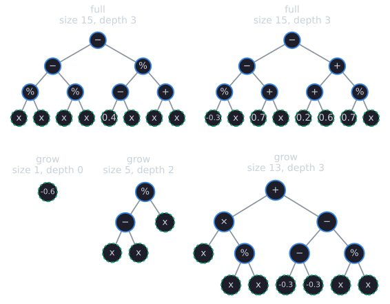
Both methods build a tree from the root down, recursively, and both stop at a maximum depth $D$, with the root at depth 0 (Poli, Langdon and McPhee, 2008, §2.2, Algorithm 2.1).
- Full chooses a function at every node above depth $D$ and a terminal at depth $D$. Every leaf therefore lies at depth $D$. When all functions have the same arity, every full tree of depth $D$ has the same size; with mixed arities sizes vary, although the range of sizes and shapes can still be rather limited (Poli, Langdon and McPhee, 2008, §2.2).
- Grow chooses each node from the whole primitive set until depth $D$, where it must choose a terminal. In the Field Guide's formulation, a node above the limit is a terminal with probability $|T|/(|T| + |F|)$, where $|T|$ and $|F|$ are the numbers of terminals and functions, so every primitive is equally likely. Branches can end early, and trees vary in shape.
Ramped half-and-half
Neither method alone gives a wide spread of shapes, so Koza (1992) combined them in ramped half-and-half: half the population is built with full and half with grow, over a range of depth limits, the "ramp" (Poli, Langdon and McPhee, 2008, §2.2). A depth range of 2 to 6 is common (Poli, Langdon and McPhee, 2008, §3.4). In the implementation used here, individual $i$ gets depth limit $2 + (i \bmod 5)$ and alternates between full and grow in blocks of five, so each depth gets 2,000 of the 10,000 trees, half from each method.
What the methods produce
The script builds 10,000 trees with each method over the primitive set {+, −, ×, %} with terminals $x$ and an ephemeral random constant on $[-1, 1)$, so $|F| = 4$ and $|T| = 2$, and grow chooses a terminal with probability 1/3:
| Method | Depth 0 | 1 | 2 | 3 | 4 | 5 | 6 | Median size | Mean size | Single node |
|---|---|---|---|---|---|---|---|---|---|---|
| Full, limits 2 to 6 | 0 | 0 | 2,000 | 2,000 | 2,000 | 2,000 | 2,000 | 31 | 48.60 | 0% |
| Grow, limit 6 | 3,367 | 725 | 362 | 214 | 134 | 91 | 5,107 | 15 | 19.33 | 33.7% |
| Ramped half-and-half, 2 to 6 | 1,637 | 368 | 1,735 | 1,647 | 1,551 | 1,526 | 1,536 | 15 | 29.69 | 16.4% |
| Ramped, grow root always a function | 0 | 550 | 2,116 | 1,920 | 1,836 | 1,801 | 1,777 | 15 | 32.15 | 0% |
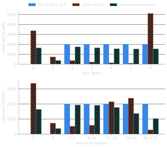
Three things stand out.
Full trees come in five sizes. With only binary functions, a full tree of depth $d$ has exactly $2^{d+1} - 1$ nodes, so the full half of the population has sizes 7, 15, 31, 63 and 127 and nothing in between.
Grow is bimodal. A third of the grow trees are a single node, because the root itself is a terminal with probability 1/3, and just over half reach the depth limit. Few lie in between. Luke (2000) explains why. If each new node has on average $g$ children, the expected number of nodes at depth $i$ is $g^i$, and without a depth limit the expected tree size is $1/(1 - g)$ when $g < 1$ and infinite otherwise. Here $g = (4/6) \times 2 = 4/3$, so an unlimited grow tree that survives its first few nodes tends to keep growing, and the depth limit cuts it off. With many terminals the balance tips the other way. With the same functions and nine terminals ($x_1, \dots, x_8$ and a constant), $g = (4/13) \times 2 = 8/13$ and the expected unlimited size is 2.6; the script measures a mean of 2.50 under the depth limit of 6, with 68.8% of trees a single node and a median size of 1. Poli, Langdon and McPhee (2008, §2.2) give the same warning in words: with many more terminals than functions, grow almost always produces very short trees, and with many more functions it behaves much like full. Small changes to the primitive set can thus change the initial population a great deal.
The same reasoning predicts the mean sizes in the table, depth limit included. Above the limit, each node grow creates is a function with probability $p = |F|/(|F| + |T|)$, and a function has $b$ children (here $b = 2$). Each node at depth $i$ therefore has on average $g = p\,b$ children at depth $i + 1$, and by induction the expected number of nodes at depth $i$ is $g^i$. At the limit $D$ every node is a terminal, so nothing lies deeper, and the expected size is the partial geometric sum
$$E[\text{size}] = \sum_{i=0}^{D} g^i = \frac{g^{D+1} - 1}{g - 1} \quad (g \neq 1).$$
For the primitive set above, $g = 4/3$ and $D = 6$ give $3\bigl((4/3)^7 - 1\bigr) = 19.47$, against the measured mean of 19.33; for the nine-terminal set, $g = 8/13$ gives 2.51, against 2.50. The full half of the ramped population has the exact mean $(7 + 15 + 31 + 63 + 127)/5 = 48.6$. The grow half has expected sizes 4.11, 6.48, 9.64, 13.86 and 19.47 at limits 2 to 6, a mean of 10.71, so the ramped population should average $(48.6 + 10.71)/2 = 29.66$ nodes; the measured mean is 29.69. (These predictions are printed by Part 5 of gp_init.py, which also checks each limit against 10,000 fresh grow trees.) The formula shows where the bimodal shape comes from: the expected size is dominated by its last terms when $g > 1$, so the mean is carried by the trees that reach the limit, while the probability $|T|/(|T| + |F|)$ that the root is a terminal fixes the share of single nodes, whatever $g$ is.
Ramped half-and-half inherits grow's small trees. In this formulation, 16.4% of the ramped population consists of single nodes, and 27.8% of the trees duplicate the shape of another tree (ignoring constant values). Forcing grow to place a function at the root (last row) removes the single-node trees and raises the mean size from 29.69 to 32.15. Koza's own implementation did not allow single-node trees and also eliminated duplicate trees (Luke, 2000). These details are rarely reported, but they change the starting population.
The size histogram of the standard ramped population is broad:
| Size | 1 | 3 | 5–7 | 9–15 | 17–31 | 33–63 | 65–127 |
|---|---|---|---|---|---|---|---|
| Trees | 1,637 | 368 | 1,929 | 1,907 | 1,768 | 1,364 | 1,027 |
Beyond ramped half-and-half
Any way of generating random programs has a bias, because there are infinitely many programs and they cannot be sampled uniformly. Ramped half-and-half favors bushy, roughly symmetric trees (Poli, Langdon and McPhee, 2008, §5.1.1). Several alternatives give more control.
Probabilistic tree creation (Luke, 2000) addresses grow's lack of control over size. PTC1 is a modified grow in which the user specifies the probability of each function and terminal and a desired expected tree size $E$; the algorithm then chooses a function rather than a terminal with probability
$$p = \frac{1 - 1/E}{\sum_{n \in N} q_n b_n},$$
where $q_n$ is the probability of function $n$ among the functions and $b_n$ is its arity. This makes $g = p \sum_n q_n b_n = 1 - 1/E$ and so the expected size exactly $E$. For four equally likely binary functions and $E = 20$, $p = 0.95/2 = 0.475$. PTC2 instead takes a whole distribution of desired sizes, draws a size from it, and builds a tree of that size or slightly larger, giving control over the spread as well as the mean. Luke shows both to be fast, effectively linear in the tree size under reasonable conditions, and gives versions of both for strongly typed GP. Other methods sample trees uniformly at random from all trees of a given size, which produces more asymmetric trees with some leaves close to the root (Poli, Langdon and McPhee, 2008, §5.1.1).
The initial distribution does not last. Crossover rearranges the sizes and shapes of the initial trees within a few generations, and initializations that produce many short programs may make bloat appear sooner (Poli, Langdon and McPhee, 2008, §5.1.2).
Subtree crossover
Subtree crossover is the standard GP recombination operator. It chooses a crossover point (a node) in each parent, independently, and replaces the subtree at the point in a copy of the first parent with a copy of the subtree at the point in the second (Poli, Langdon and McPhee, 2008, §2.4). The parents are copied so that a parent selected several times is not changed. The common form produces one child; a version that also returns the complementary child exists but is less used. Swapping the roles of the parents in the opening example gives the complementary child (* (- x 1) (% x 2)).
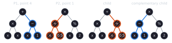
Unlike GA crossover, which exchanges values at matching positions, subtree crossover can move code to a different position, depth and context, and it changes the size of the child: the child's size is the first parent's size minus the removed subtree plus the inserted one. In the opening example both exchanged subtrees have three nodes, so the sizes do not change; choosing the root of P2 (all seven nodes) as the inserted subtree and the leaf x at node 2 of P1 as the point gives a child of $7 - 1 + 7 = 13$ nodes and depth 4, (+ (* (* (+ x 0.5) (% x 2)) x) (- x 1)).
The demo makes three properties easy to check. Choosing a leaf in P1 and the root of P2 grows the child by the whole of P2, minus one node. Choosing the root of P1 returns a copy of P2's chosen subtree, so the child can be as small as a single node. And choosing two identical subtrees, such as an x in each parent, returns P1 unchanged, which is how crossover between the article's two parents can produce a child identical to its first parent.
The 90/10 rule
Choosing crossover points uniformly over all nodes has a problem: most nodes are leaves. A tree built only from binary functions with $n$ function nodes has $n + 1$ leaves, more than half its nodes, and a tree of size 1 is all leaf. (Count the edges two ways: every node except the root hangs from exactly one edge, so a tree with $n$ function nodes and $L$ leaves has $n + L - 1$ edges, and every function node has exactly two edges below it, so there are $2n$. Equating the two gives $L = n + 1$.) In the ramped population above, leaves make up 61.5% of the nodes of the average tree (51.7% of all nodes pooled, because large trees have proportionally fewer). With uniform selection, about 38% of crossovers would exchange one leaf for another, often a terminal for an identical terminal. To make crossover exchange larger pieces of code, Koza (1992) suggested choosing function nodes 90% of the time and leaves 10% of the time, a rule that is still widely used (Poli, Langdon and McPhee, 2008, §2.4). Averaged over the ramped population, the expected size of the selected subtree is 3.39 nodes under uniform selection and 5.55 under the 90/10 rule.
The rule is a parameter like any other. Angeline (1996) varied the leaf selection frequency in subtree crossover, in a non-standard GP system, and reported that performance was sensitive to it and could often be improved by setting the frequency by a random process rather than a constant.
Depth limits
Subtree crossover can produce children much deeper than either parent, so GP systems impose a maximum depth or size. A common implementation, used by Koza (1992), applies the operator and, if the child exceeds the limit, returns a parent instead (Poli, Langdon and McPhee, 2008, §11.3.2). Luke and Spector (1997), keeping close to Koza's traditional settings, used a depth limit of 17. Returning parents has side effects, such as filling the population with trees that sit just under the limit; bloat in genetic programming discusses these and the alternatives.
Mutation operators
GP uses many mutation operators, often several at once (Poli, Langdon and McPhee, 2008, §5.2.2). Applied to P1 = (+ (* x x) (- x 1)):
| Operator | What it does | Example result |
|---|---|---|
| Subtree mutation | Replaces a randomly chosen subtree with a new random tree | (* x x) replaced by (% x (+ x x)): (+ (% x (+ x x)) (- x 1)) |
| Point mutation | Replaces a node with a different primitive of the same arity, keeping its children | * replaced by %: (+ (% x x) (- x 1)) |
| Hoist mutation | Returns a copy of a randomly chosen subtree of the parent | (- x 1) |
| Shrink mutation | Replaces a randomly chosen subtree with a random terminal | (* x x) replaced by x: (+ x (- x 1)) |
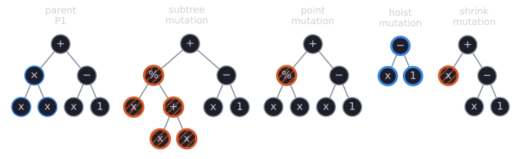
Subtree mutation is Koza's mutation (Koza, 1992, p. 106, as cited by Poli, Langdon and McPhee, 2008, §5.2.2). The new subtree is usually generated with grow or full and a small depth limit. It can be implemented as crossover with a freshly generated random tree, sometimes called "headless chicken" crossover (Poli, Langdon and McPhee, 2008, §2.4).
Point mutation, or node replacement mutation, is the nearest GP analogue of the bit-flip mutation of genetic algorithms. It is usually applied per node: each node, with some probability, is replaced by a different primitive with the same number of arguments, and if no such primitive exists the node is left alone (Poli, Langdon and McPhee, 2008, §2.4). It never changes a tree's size or shape.
Hoist mutation and shrink mutation both make trees smaller. Poli, Langdon and McPhee (2008, §5.2.2) attribute hoist to Kinnear (1994) and shrink to Angeline (1996); both are motivated by the wish to reduce program size. Other operators in the same catalogue permute a function's arguments, perturb numerical constants with Gaussian noise, or optimize the constants by local search.
What each operator does to size
The script applies each operator to the same 10,000 parents (pairs, for crossover) drawn at random from the ramped half-and-half population; the drawn parents have mean size 29.62. The new subtree in subtree mutation is a grow tree of depth at most 4, at a uniformly chosen point:
| Operator | Mean child size | Change | Larger | Smaller | Identical to parent |
|---|---|---|---|---|---|
| Subtree crossover, 90/10 | 29.65 | +0.03 | 37.1% | 37.2% | 1.7% |
| Subtree crossover, uniform points | 29.74 | +0.11 | 28.2% | 28.3% | 9.7% |
| Subtree mutation | 35.96 | +6.33 | 61.1% | 16.5% | 5.0% |
| Point mutation, rate 0.1 per node | 29.62 | 0.00 | 0% | 0% | 39.1% |
| Hoist mutation | 2.67 | −26.96 | 0% | 83.6% | 16.4% |
| Shrink mutation | 24.52 | −5.10 | 0% | 83.6% | 16.4% |
Crossover leaves the mean size unchanged, as it must when both parents come from the same population: on average the inserted subtree is as large as the removed one. Uniform point selection makes 9.7% of crossovers return an exact copy of the first parent, mostly by swapping a terminal for an identical one; the 90/10 rule cuts that to 1.7%. Subtree mutation grows trees on average here, because a uniformly chosen point is usually a leaf and the replacement is usually larger. Hoist and shrink can only shrink trees; the 16.4% of identical children are the single-node parents, which they leave unchanged. Hoist's effect is drastic, from 29.62 nodes to 2.67 on average, for the same reason that uniform crossover points tend to be leaves: in this implementation the hoisted subtree is chosen uniformly among the non-root nodes, and most nodes of a tree are leaves or sit just above them. These are measurements of one application of each operator to a random population, not of a run. Under selection, sizes change in ways these averages do not predict, which is the subject of bloat.
Operator rates
In GP the operators are usually mutually exclusive: each child is produced by exactly one of them, chosen at random with given probabilities. Traditionally crossover is applied at a rate of 90% or more and mutation at around 1%, with reproduction, copying a selected individual unchanged, filling the remainder (Poli, Langdon and McPhee, 2008, §2.4). A 50–50 mixture of crossover and several mutations also appears to work well (Poli, Langdon and McPhee, 2008, §3.4).
Crossover versus mutation in GP
Koza (1992) used no mutation in most of his experiments. Poli, Langdon and McPhee (2008, §5.2.1) report that he wanted to show that mutation was not necessary and that GP was not a simple random search, and that this choice strongly influenced the field. Luke and Spector (1997) summarize his argument as resting on the position independence of GP subtrees and the large number of positions in a typical population (Koza, 1992, pp. 105–107), supported by data from one problem, the Boolean 6-multiplexer (pp. 599–600).
Luke and Spector (1997) tested the claim systematically. They compared 90% crossover against 90% subtree mutation, each with 10% reproduction, on four problems (the 6-multiplexer, the lawnmower, symbolic regression of $x^4 + x^3 + x^2 + x$, and the artificial ant on the Santa Fe trail), over a grid of population sizes and run lengths, with tournament sizes 2 and 7, a depth ramp of 2 to 6 and a depth limit of 17. Their subtree mutation, which they called "point" mutation, picked internal nodes 90% of the time. They found crossover more successful in the majority of tests, mutation tending to do better with smaller populations and more generations, few large differences between the two, and, in most situations, a larger effect from changing the tournament size, and with it the selection pressure, than from choosing crossover over mutation. A second set of runs found no blend of the two that was consistently and significantly better than either alone.
The study had two statistical flaws, which the authors corrected the following year (Luke and Spector, 1998): the results for different run lengths had been read from the same runs as they continued, so they were not independent, and 25 runs per setting were too few. The revision repeated the crossover-versus-mutation comparison (not the blends) with 50 independent runs per setting and three times as much computation, about 1.67 billion evaluations. Its conclusions were similar. Crossover was more successful overall; even where the difference was statistically significant, it was often surprisingly small, except in symbolic regression; changing the tournament size often mattered more; and the trend that mutation did better in small populations and crossover in large ones was obvious only in symbolic regression and the 6-multiplexer. The authors concluded that crossover does something useful beyond acting as an unusual mutation, but that its extra benefit is usually modest, and that which operator is preferable depends strongly on the problem and the parameters. Poli, Langdon and McPhee (2008, §5.2.1) summarize the wider literature the same way: mutation-based search, alone or combined with hill climbing or simulated annealing, has matched or beaten crossover-based GP on some problems, and the relative performance depends on the problem and the details of the system. Mutation is now widely used.
The script gp_xo_vs_mut.py repeats the comparison on a small scale, as a check rather than a replication: the same quartic symbolic regression target at 20 evenly spaced points in $[-1, 1]$, {+, −, ×, %} with terminal $x$ and no constants, tournament size 7, 90% of one operator plus 10% reproduction, 90/10 node selection for both operators, depth limit 17, and 50 generations, with 30 seeded runs per setting. A run "hits" if its best program is within 0.01 of the target at all 20 points.
| Population | Operator | Best-of-run error, median [Q1, Q3] | Runs that hit all 20 cases | Final mean tree size (median) |
|---|---|---|---|---|
| 50 | 90% crossover | 0.0000 [0.0000, 4.7237] | 19 of 30 | 15.6 |
| 50 | 90% subtree mutation | 0.0000 [0.0000, 1.1108] | 17 of 30 | 210.7 |
| 500 | 90% crossover | 0.0000 [0.0000, 0.0000] | 30 of 30 | 116.7 |
| 500 | 90% subtree mutation | 0.0000 [0.0000, 0.0000] | 28 of 30 | 259.0 |
On this easy problem both operators usually find the target exactly, and the differences in hits, two runs of 30 at each population size, are too small to separate with 30 runs. At population 50 the runs that failed did worse with crossover (upper quartile 4.72) than with mutation (1.11). The clearest difference in our runs is not in fitness but in size: the mutation runs ended with much larger trees, 210.7 and 259.0 nodes against 15.6 and 116.7, and so took much longer to evaluate. Luke and Spector (1998) remarked, anecdotally, that tree growth seemed to waste more time in their crossover runs; in this smaller setup, with its particular mutation settings, the reverse happened. One problem and two population sizes cannot settle the question, which is the point of the larger studies: the answer depends on the problem, the population size and details such as how new subtrees are generated.
References
- Angeline, P. J. (1996). An investigation into the sensitivity of genetic programming to the frequency of leaf selection during subtree crossover. In J. R. Koza, D. E. Goldberg, D. B. Fogel, and R. L. Riolo (eds.), Genetic Programming 1996: Proceedings of the First Annual Conference, 21–29. MIT Press.
- Eiben, A. E., and Smith, J. E. (2015). Introduction to Evolutionary Computing, 2nd ed., sections 4.6 and 6.4. Springer.
- Kinnear, K. E., Jr. (1994). Fitness landscapes and difficulty in genetic programming. In Proceedings of the First IEEE Conference on Evolutionary Computation (IEEE World Congress on Computational Intelligence), vol. 1, 142–147. IEEE.
- Koza, J. R. (1992). Genetic Programming: On the Programming of Computers by Means of Natural Selection. MIT Press.
- Luke, S. (2000). Two fast tree-creation algorithms for genetic programming. IEEE Transactions on Evolutionary Computation, 4(3), 274–283.
- Luke, S., and Spector, L. (1997). A comparison of crossover and mutation in genetic programming. In J. R. Koza et al. (eds.), Genetic Programming 1997: Proceedings of the Second Annual Conference, 240–248. Morgan Kaufmann.
- Luke, S., and Spector, L. (1998). A revised comparison of crossover and mutation in genetic programming. In J. R. Koza et al. (eds.), Genetic Programming 1998: Proceedings of the Third Annual Conference, 208–213. Morgan Kaufmann.
- Poli, R., Langdon, W. B., and McPhee, N. F. (2008). A Field Guide to Genetic Programming. Published via lulu.com, freely available at gp-field-guide.org.uk (with contributions by J. R. Koza).