The expression $x^2 + x + 1$ can be written as a tree. The root is an addition; its left child is a multiplication of $x$ by $x$, and its right child is another addition, of $x$ and 1. In the bracketed prefix notation of Lisp the same tree reads
(+ (* x x) (+ x 1))
and it is a small computer program: given a value of $x$, evaluating the tree from the leaves up returns a number. Genetic programming (GP) is an evolutionary algorithm whose individuals are programs like this one. It creates a population of random trees, runs each one on a set of test inputs, scores how close its outputs come to what is wanted, and breeds the better trees by exchanging and replacing their subtrees. Over many generations the population can arrive at a program, such as the tree above, that nobody wrote.
This article describes the representation: what a program tree is, the sets of primitives it is built from, the properties those sets need, and how a tree-based search differs from a genetic algorithm on fixed-length strings. How the first trees are created and how they are varied is the subject of initialization and variation in genetic programming. The main modern source is the free A Field Guide to Genetic Programming by Poli, Langdon and McPhee (2008), cited here by section; the textbook treatment is Eiben and Smith (2015, §4.6 and §6.4). Every number below is printed by tools/experiments/evolution/gp_trees.py in the site repository, which uses the small GP library tools/experiments/evolution/gp.py.
What genetic programming evolves
The idea of evolving programs is older than GP. Cramer (1985) presented two small languages for evolving programs at the first International Conference on Genetic Algorithms; in the second, programs were trees and crossover exchanged subtrees. Koza developed the tree representation into a general method and demonstrated it on a wide range of problems in Genetic Programming: On the Programming of Computers by Means of Natural Selection (Koza, 1992). The history of evolutionary computation places this work among the other branches of the field.
In practice GP rarely evolves programs in a general-purpose language. It evolves expressions in a small, problem-specific language whose words are chosen by the user: arithmetic for fitting a formula to data, Boolean operators for a logic circuit, movement commands for a simulated robot (Poli, Langdon and McPhee, 2008, §3.1). One of the earliest and most widely used applications, fitting a formula to data, is called symbolic regression.
Program trees and prefix notation
A program tree has two kinds of node. Functions are internal nodes: operations such as $+$, $\times$, $\sin$ or IF, each with a fixed number of arguments, its arity. Terminals are leaves: input variables such as $x$, constants such as 1, and functions of no arguments, such as a sensor reading. The functions and terminals together make up the primitive set (Poli, Langdon and McPhee, 2008, §2.1).
Two measures of a tree recur throughout GP. The depth of a node is the number of edges between it and the root, so the root has depth 0, and the depth of a tree is the depth of its deepest node. The size of a tree is its number of nodes. For the example tree:
| Notation | Form |
|---|---|
| Prefix (S-expression) | (+ (* x x) (+ x 1)) |
| Linear prefix | + * x x + x 1 |
| Infix | ((x * x) + (x + 1)) |
| Nodes in preorder, with depths | +@0, *@1, x@2, x@2, +@1, x@2, 1@2 |
The tree has size 7 and depth 2. Prefix notation mirrors the tree directly: each pair of brackets is a subtree, and its first symbol is that subtree's root. When every function has a fixed arity the brackets are redundant, because the arity of each symbol says how many of the following subexpressions belong to it, so a tree can be stored as the flat sequence + * x x + x 1 (Poli, Langdon and McPhee, 2008, §2.1). Many GP systems store trees this way, as a flat array in preorder, because it is compact and fast to copy. The same idea, a tree serialized so that operators precede their operands, appears in the query trees that a search engine builds from a Boolean query.
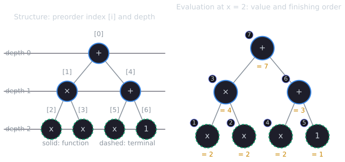
A useful habit when reading GP output is to translate between the three forms. The bracketed prefix form is the tree read top-down; the infix form is what a person would write; the preorder index of a node is its position in the flat sequence, and it is how the operators described in initialization and variation in genetic programming address crossover and mutation points. In the left panel, the subtree rooted at index 4 occupies indices 4 to 6, a contiguous block of the flat sequence. Every subtree is contiguous in preorder, which is why a subtree can be cut out of, or spliced into, a flat array with one slice.
Running a tree
A tree is run by an interpreter that evaluates each node after its arguments, usually by a recursive traversal from the root (Poli, Langdon and McPhee, 2008, §3.3, Algorithm 3.1). The call on the root asks for the values of its two children, each child asks for its own children's values, and the recursion bottoms out at the leaves. Values then flow back up. At $x = 2$, nodes finish in this order (printed by Part 8 of the script):
| Finishes | Node (preorder index) | Arguments | Returns |
|---|---|---|---|
| 1 | x [2] |
2 | |
| 2 | x [3] |
2 | |
| 3 | * [1] |
2, 2 | 4 |
| 4 | x [5] |
2 | |
| 5 | 1 [6] |
1 | |
| 6 | + [4] |
2, 1 | 3 |
| 7 | + [0] |
4, 3 | 7 |
The output is $7 = 2^2 + 2 + 1$. The finishing order is a postorder traversal: every node appears after all of its descendants.
The flat preorder array can be run without recursion and without brackets. Scan it from right to left with a stack: a terminal pushes its value, and a function of arity $k$ pops $k$ values (the first popped is its first argument), applies itself, and pushes the result.
| Read | Stack afterwards (top at right) |
|---|---|
1 |
1 |
x |
1, 2 |
+ |
3 |
x |
3, 2 |
x |
3, 2, 2 |
* |
3, 4 |
+ |
7 |
Each function finds exactly its arguments on top of the stack because, read backward, a subtree's arguments are complete before its root is reached. This is the reason fixed arities make the brackets redundant, and it is the evaluation scheme that stack-based GP adopts as its representation, with the program written in postfix order and read left to right (see genetic programming beyond trees).
For functions without side effects the order of evaluation among siblings does not matter. For functions with side effects, such as a robot's MOVE, it does, and the interpreter can treat some primitives as macros that receive their arguments unevaluated, so that a conditional, for example, runs only the branch it chooses.
Function and terminal sets
The first two decisions in any GP application are the terminal set and the function set, because together they define the language in which every candidate program is written. Typical choices (after Poli, Langdon and McPhee, 2008, Table 3.1):
| Kind | Examples |
|---|---|
| Arithmetic functions | $+$, $-$, $\times$, protected $\div$ |
| Mathematical functions | $\sin$, $\cos$, $\exp$ |
| Boolean functions | AND, OR, NOT |
| Conditionals and loops | IF-THEN-ELSE, REPEAT |
| Terminals | input variables, constants, zero-argument functions such as rand or a sensor |
Constants need special handling, because a fixed list of constants rarely contains the value a problem needs. The usual device is the ephemeral random constant: a terminal symbol that, each time it is chosen while building a tree, is replaced by a freshly drawn random number, which then stays fixed in that tree for the rest of the run (Poli, Langdon and McPhee, 2008, §3.1). Evolution can then build other values by arithmetic on these.
Two properties of the primitive set decide whether GP can work with it at all: closure and sufficiency.
Closure
GP's operators cut and splice trees without regard to meaning. Subtree crossover can move any subtree into any argument position of any function. For every resulting tree to be a valid program, the primitive set needs closure (Koza, 1992), which Poli, Langdon and McPhee (2008, §3.2.1) divide into two parts.
Type consistency requires that every function accept, in every argument, any value that any function or terminal can return. The simplest way to achieve it is to use a single type throughout, such as floating-point numbers.
Evaluation safety requires that every function return a usable value for every input. Division fails when the divisor is 0, and the logarithm fails for non-positive arguments. GP systems therefore use protected versions that check their inputs and return a default value instead of failing. Protected division, often written %, typically returns 1 when the divisor is 0 (Poli, Langdon and McPhee, 2008, §3.2.1):
| Expression | Value |
|---|---|
(% x (- x x)) at $x = -2$, 0 and 3.5 |
1, 1, 1 |
x / (x - x) in plain Python at $x = 3.5$ |
ZeroDivisionError |
The choice of 1 is not arbitrary: it lets GP build the constant 1 as (% x x), just as (- x x) builds 0. In the fitness-case table below, the tree (+ (% x x) (* x (+ x 1))) matches the target exactly at $x = 0$ only because the protected division returns 1 there.
Protection has a cost. It hides the singularity only at exactly 0; next to it the function behaves as ordinary division. The script evaluates (% 1 (- x 0.3)) near $x = 0.3$:
| $x$ | 0.29 | 0.2999 | 0.3 | 0.3001 | 0.31 |
|---|---|---|---|---|---|
| value | $-100$ | $-10{,}000$ | 1 | 10,000 | 100 |
An evolved formula can therefore contain a pole that happens to fall between the fitness cases, fit the data, and return enormous values on new inputs. This is one reason symbolic regression checks evolved models on data not used for fitness. The alternative to protection is to let errors occur and give any program that causes one a very poor fitness, but when invalid programs are common this leaves many individuals with nearly the same poor fitness and gives selection little to work with (Poli, Langdon and McPhee, 2008, §3.2.1).
Types and strongly typed GP
A single type is not always natural. A conditional needs a Boolean test, and a numeric program may still want comparisons. Consider the absolute value written with a three-argument IF:
P1 = (if (> x 0) x (- 0 x))
Here > returns a Boolean, if needs a Boolean first argument and numbers for the other two, and everything else is numeric. The script performs every possible subtree crossover between P1 and P2 = (+ x 1), in both directions: 48 pairs of crossover points. Six of the children are ill-typed, among them (if (+ x 1) x (- 0 x)), with a number where the test should be, (+ (> x 0) 1), with a Boolean added to a number, and the bare (> x 0), a Boolean where the program should return a number.
There are three standard remedies (Poli, Langdon and McPhee, 2008, §3.2.1 and §6.2.2). The first converts automatically between types, for example by treating negative numbers as false, at the risk of introducing biases. The second restructures the function set so that one type suffices; the four-argument IFLTE, "if $a < b$ then $c$ else $d$", does the work of IF and $<$ with numbers only, and (iflte x 0 (- 0 x) x) computes $|x|$. The third is strongly typed genetic programming (STGP), introduced by Montana (1995). Every terminal has a type, every function has types for its arguments and its return value, and tree creation and every operator respect them: crossover may only swap subtrees whose roots return the type expected at the insertion point. Of the 48 pairs above, STGP allows 42, and all 42 yield well-typed children. Montana noted that this basic form is close to the "constrained syntactic structures" of Koza (1992, ch. 19), which specify directly which children each function may have; his main additions were generic functions, such as a single MATRIX-ADD that adds any two matrices of the same shape, and generic data types. His motivation was that, without type constraints, programs that manipulate several data types can need unnecessarily long searches and generalize unnecessarily poorly. Grammar-based GP extends the same idea from types to grammars (Poli, Langdon and McPhee, 2008, §6.2.3).
Sufficiency
Closure guarantees that every tree runs. Sufficiency asks whether some tree solves the problem: the primitive set is sufficient if a solution can be expressed by composing its primitives (Poli, Langdon and McPhee, 2008, §3.2.2). Sometimes theory settles the question. {AND, OR, NOT} with the input variables can express every Boolean function, so it is sufficient for any Boolean problem. {+, −, ×, ÷} with $x$ and a few integer constants is not sufficient for $e^x$: every tree over it computes a rational function of $x$, and $e^x$ is not one. GP with that set can only approximate $e^x$, although the approximation may be good enough.
For most real problems sufficiency cannot be guaranteed, and the user's choice of primitives encodes a guess about the form of the answer. Adding primitives makes sufficiency more likely but enlarges the search space; Poli, Langdon and McPhee (2008, §3.2.2) report that a few unnecessary primitives do not tend to slow GP down much, although they can bias it in unexpected ways.
Fitness cases and the preparatory steps
A program's fitness usually depends on its behavior over many inputs or situations, called fitness cases. For the target $x^2 + x + 1$, five fitness cases at $x = -1, -0.5, 0, 0.5, 1$ and fitness defined as the sum of absolute errors give:
| Program | $-1$ | $-0.5$ | 0 | 0.5 | 1 | Error |
|---|---|---|---|---|---|---|
| target $x^2 + x + 1$ | 1.00 | 0.75 | 1.00 | 1.75 | 3.00 | |
(+ x 1) |
0.00 | 0.50 | 1.00 | 1.50 | 2.00 | 2.50 |
(* x (+ x 1)) |
0.00 | −0.25 | 0.00 | 0.75 | 2.00 | 5.00 |
(+ (* x x) 1) |
2.00 | 1.25 | 1.00 | 1.25 | 2.00 | 3.00 |
(+ (% x x) (* x (+ x 1))) |
1.00 | 0.75 | 1.00 | 1.75 | 3.00 | 0.00 |
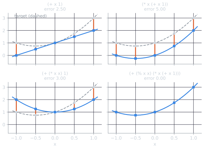
The second and third programs each contain part of the answer, $x(x+1)$ and $x^2 + 1$, but score worse than the cruder (+ x 1). The figure shows why. (* x (+ x 1)) has exactly the right shape and is wrong by the same amount, 1, at every case, so its five errors add up to 5. (+ (* x x) 1) is exact at $x = 0$ but misses the linear term, which costs $\lvert x \rvert$ at each case, a total of 3. (+ x 1) misses the quadratic term instead, which costs $x^2$, small near the middle of the interval: $1 + 0.25 + 0 + 0.25 + 1 = 2.5$. Fitness rewards behavior, not the presence of useful parts, which is why the way GP recombines parts matters: a crossover that replaces the x of a parent (+ 1 x) with the (* x (+ x 1)) of another produces the target, but nothing in either parent's fitness says which parts to keep.
Setting up a GP run is conventionally described as a short list of preparatory steps, which Poli, Langdon and McPhee (2008, ch. 3) give as five decisions:
- the terminal set;
- the function set;
- the fitness measure, including the fitness cases;
- the parameters that control the run, such as population size, operator probabilities and limits on tree size;
- the termination criterion and the method of designating the result, typically the best program found.
The first two define the space of programs, the third says which programs in it are good, and the last two control the search.
How big trees can get
The size of a tree is bounded by its depth and by the arities of its functions. If the largest arity is $a \geq 2$, a tree of depth $d$ has at most $a^i$ nodes at depth $i$, so its size is at most
$$\sum_{i=0}^{d} a^i = \frac{a^{d+1} - 1}{a - 1}.$$
The familiar bound $2^{d+1} - 1$ is the case $a = 2$, and it holds only when no function takes more than two arguments. A function set containing a three-argument IF raises the bound to $(3^{d+1} - 1)/2$. In the other direction, a tree of depth exactly $d$ contains a path of $d$ function nodes from the root to its deepest leaf, and the smallest such tree fills every other argument of those nodes with a terminal. If the smallest arity is $m$, its size is at least $1 + md$:
| Depth $d$ | 0 | 1 | 2 | 3 | 4 | 5 | 6 |
|---|---|---|---|---|---|---|---|
| Maximum size, largest arity 2 | 1 | 3 | 7 | 15 | 31 | 63 | 127 |
| Maximum size, largest arity 3 | 1 | 4 | 13 | 40 | 121 | 364 | 1093 |
| Minimum size, smallest arity 2 | 1 | 3 | 5 | 7 | 9 | 11 | 13 |
| Minimum size, smallest arity 1 | 1 | 2 | 3 | 4 | 5 | 6 | 7 |
With mixed arities even a full tree, one whose leaves all lie at the same depth, has no fixed size. The script draws 10,000 full trees of depth 4 over {+, −, ×, %, sin, cos}, four binary functions and two unary ones. Their sizes range from 5 to 31, the two bounds, with median 18 and mean 17.83. Each function node has $b = (4 \cdot 2 + 2 \cdot 1)/6 = 5/3$ children on average, so the expected size is $\sum_{i=0}^{4} b^i = 17.79$, in line with the sample.
The number of distinct trees grows far faster. The count follows from one observation: a tree of depth at most $d$ is either a single terminal, or a function whose every argument is a tree of depth at most $d - 1$. The two cases do not overlap, and in the second the arguments can be chosen independently. With $|T|$ terminals and the function set $F$, the number $N_d$ of trees of depth at most $d$ therefore satisfies
$$N_0 = |T|, \qquad N_d = |T| + \sum_{f \in F} N_{d-1}^{\,\mathrm{arity}(f)}.$$
For {+, −, ×, %} and {$x$, 1}, $|T| = 2$ and there are four binary functions, so $N_d = 2 + 4 N_{d-1}^2$. Step by step: $N_1 = 2 + 4 \cdot 2^2 = 18$ (the two terminals and the $4 \times 2 \times 2 = 16$ trees such as (+ x 1)), $N_2 = 2 + 4 \cdot 18^2 = 1{,}298$, and $N_3 = 2 + 4 \cdot 1{,}298^2 = 6{,}739{,}218$. Because the previous count is squared at every step, $\log N_d$ roughly doubles with each extra level of depth:
| Depth at most | 0 | 1 | 2 | 3 | 4 |
|---|---|---|---|---|---|
| Distinct trees | 2 | 18 | 1,298 | 6,739,218 | about $1.8 \times 10^{14}$ |
| Distinct functions they compute | 2 | 10 | 131 | 14,494 |
Many of these trees compute the same function. The last row, from Part 9 of the script, counts the different functions: two trees are counted once if their values at eight fixed values of $x$, computed exactly in rational arithmetic, are equal. Of the 18 trees of depth at most 1, (+ x 1) and (+ 1 x) compute the same function, (- x x) and (- 1 1) both compute 0, and (* x 1), (% x 1) and x all compute $x$; after all such merges, 10 functions remain. At depth 3, about 465 trees on average compute each distinct function. (The count at depth 4 is beyond this simple method: it would combine every pair of the 14,494 depth-3 functions under four operators.) This redundancy is part of what makes GP's search space easier than its raw size suggests: a search that reaches a function can reach it through many trees.
Even so, the count shows why GP cannot enumerate even shallow programs and why limits on depth or size are part of every practical system. Without them, trees tend to grow during a run without improving fitness, the problem of bloat.
How GP differs from a genetic algorithm
GP uses the same loop as every evolutionary algorithm: a population, selection by fitness, variation, repetition. The representation changes almost everything else.
- Variable size and shape. A genetic algorithm's genome is a string of fixed length, and position $i$ always encodes the same variable. A program tree has no fixed length or shape, and its size typically changes during a run. The search is over structures as well as values.
- Operators on subtrees. Crossover in a GA exchanges the values at corresponding positions. GP's subtree crossover removes a subtree from one parent and inserts a subtree from the other, from any position, at the chosen point. The operators are described in initialization and variation in genetic programming.
- No fixed positions. Because a subtree can move to a different place in the tree, the meaning of a piece of code depends on its context. A GA crossover of a string with itself, such as 11010011 with 11010011, returns the parent at every cut point. Crossing
(+ (* x x) (+ x 1))with itself, over all 49 pairs of crossover points, gives 29 different children, of sizes from 1 to 13, among them(+ (+ x 1) (+ x 1))and the single nodex; only 13 of the 49 pairs return the parent. Crossover in GP can therefore keep creating new programs even in a population of identical trees. Whether it does more than a large random mutation has been debated, and the next article summarizes the evidence. - Genotype and phenotype coincide. The tree is both what is varied and what is run. There is no decoding step, unlike the binary encodings of a GA.
- Theory. The schema theorem counts patterns at fixed string positions, which tree representations do not have. GP schema theories exist, but they define schemata over tree shapes and positions and are considerably more complicated (Poli, Langdon and McPhee, 2008, §11.1).
The same variable-structure problem returns in NEAT, which evolves neural networks whose topology grows, and in compositional pattern-producing networks, which generate patterns by composing simple functions, much as a GP tree does.
References
- Cramer, N. L. (1985). A representation for the adaptive generation of simple sequential programs. In J. J. Grefenstette (ed.), Proceedings of the First International Conference on Genetic Algorithms and Their Applications, 183–187. Lawrence Erlbaum.
- Eiben, A. E., and Smith, J. E. (2015). Introduction to Evolutionary Computing, 2nd ed., sections 4.6 and 6.4. Springer.
- Koza, J. R. (1992). Genetic Programming: On the Programming of Computers by Means of Natural Selection. MIT Press.
- Montana, D. J. (1995). Strongly typed genetic programming. Evolutionary Computation, 3(2), 199–230.
- Poli, R., Langdon, W. B., and McPhee, N. F. (2008). A Field Guide to Genetic Programming. Published via lulu.com, freely available at gp-field-guide.org.uk (with contributions by J. R. Koza).