Okapi BM25 ("Best Match 25") is a ranking function for keyword search. It scores a document by summing, over the query terms it contains, a weight that combines how rare the term is in the collection, how often it occurs in the document, and how long the document is relative to the average. It was developed by Stephen Robertson, Steve Walker, and colleagues for the Okapi system at City University London and reached its standard form at TREC-3 in 1994 (Robertson and colleagues, 1995). It is the default similarity in Lucene, and therefore in Elasticsearch, OpenSearch, and Solr. Thirty years later it is still the baseline that new retrieval methods are measured against, and it has often beaten neural retrievers on collections they were not trained for.
From BIM to BM25
The Binary Independence Model derives a principled term weight, but it sees only whether a term is present. Two things it ignores matter a great deal:
- Term frequency. A review that uses mystery twelve times is more likely to be about mysteries than one that uses it once.
- Document length. A long document contains more terms simply because it is long, so raw counts favor it unfairly.
The obvious fix, multiplying the weight by raw term frequency, overcorrects: the twelfth occurrence of a word is not twelve times as informative as the first. Robertson and Walker's route to a better function went through the 2-Poisson model, in which documents are either elite for a term, actually about its concept, or not, and term counts follow a different Poisson distribution in each group. The full model has too many parameters to estimate, so Robertson and Walker (1994) designed a simple function with the same shape: it starts at zero, rises with term frequency, and levels off at an asymptote. That function is the heart of BM25.
Building the formula in four steps
Robertson and Zaragoza (2009, §3.4.4 to §3.4.5) present the construction in a sequence of small steps, each fixing one problem. Following it makes every part of the final formula explicit.
- Start from the binary weight. The BIM gives each matching term a weight $w^{\mathrm{RSJ}}_t$, the Robertson–Spärck Jones weight, which without relevance information is an IDF. The 2-Poisson model says this is the weight a term should approach when the document is certainly elite for it.
- Saturate. Multiply by a function of term frequency that is 0 at $\mathit{tf} = 0$, increases, and approaches 1. The one-parameter function chosen was $\mathit{tf}/(\mathit{tf} + k_1)$, giving the early form $\frac{\mathit{tf}}{k_1 + \mathit{tf}}\, w^{\mathrm{RSJ}}_t$ (their eq. 3.11). It approaches the binary weight from below as $\mathit{tf}$ grows.
- Normalize length before saturating. Divide the raw count by a length factor $B = (1 - b) + b \, L_d / L_{\mathrm{avg}}$ to get $\mathit{tf}' = \mathit{tf} / B$, and saturate that instead. Substituting and multiplying top and bottom by $B$: $$\frac{\mathit{tf}'}{k_1 + \mathit{tf}'} = \frac{\mathit{tf} / B}{k_1 + \mathit{tf}/B} = \frac{\mathit{tf}}{\mathit{tf} + k_1 B}.$$ Length enters only as a rescaling of $k_1$: a long document ($B > 1$) needs more occurrences to reach the same fraction of the maximum (their eqs. 3.12 to 3.15).
- Rescale so one occurrence keeps the binary weight. Multiplying by the constant $k_1 + 1$ makes the factor exactly 1 when $\mathit{tf} = 1$ and $L_d = L_{\mathrm{avg}}$, so a single occurrence in an average document scores what the BIM would give it, and the maximum becomes $k_1 + 1$ times that. The constant is the same for every term and document, so it changes no ranking; it only keeps scores on a familiar scale.
The scoring function
For a query $q$ and document $d$:
$$\mathrm{BM25}(d, q) = \sum_{t \in q} \mathrm{IDF}(t) \cdot \frac{\mathrm{tf}_{t,d} \, (k_1 + 1)}{\mathrm{tf}_{t,d} + k_1 \left(1 - b + b \, \frac{L_d}{L_{\mathrm{avg}}}\right)}$$
| Symbol | Meaning |
|---|---|
| $\mathrm{tf}_{t,d}$ | Number of times term $t$ occurs in document $d$ |
| $L_d$, $L_{\mathrm{avg}}$ | Length of $d$ and the average document length, in tokens |
| $\mathrm{IDF}(t)$ | Rarity of $t$ in the collection, discussed below |
| $k_1$ | Controls how quickly term frequency saturates, typically 1.2 to 2.0 |
| $b$ | Controls the strength of length normalization, from 0 to 1, typically 0.75 |
Terms absent from the document have $\mathrm{tf} = 0$ and contribute nothing, so like the BIM the score can be accumulated directly from the postings lists of an inverted index.
Term frequency saturation
Write $K = k_1 \left(1 - b + b \, L_d / L_{\mathrm{avg}}\right)$. The term frequency component is then $\frac{\mathrm{tf}\,(k_1 + 1)}{\mathrm{tf} + K}$. It is zero when $\mathrm{tf} = 0$, increases with every additional occurrence, and approaches $k_1 + 1$ as $\mathrm{tf}$ grows without bound. The factor $(k_1 + 1)$ in the numerator is a normalization: for a document of average length, a single occurrence scores exactly 1. With $k_1 = 1.2$ and an average-length document:
| tf | 1 | 2 | 3 | 5 | 10 | 20 | limit |
|---|---|---|---|---|---|---|---|
| Component | 1.00 | 1.38 | 1.57 | 1.77 | 1.96 | 2.08 | 2.20 |
The second occurrence adds 0.38, the tenth adds very little. This diminishing return makes the score hard to inflate by repeating a keyword. The parameter $k_1$ sets the curve's shape. At $k_1 = 0$ the component is 1 for any $\mathrm{tf} > 0$, which recovers the binary model. As $k_1$ grows the curve approaches raw term frequency.
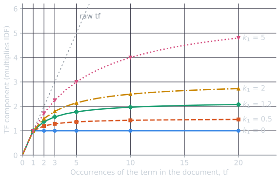
Half of the maximum is reached when $\mathrm{tf} = K$, which gives $k_1$ a direct reading: for an average-length document it is the number of occurrences at which a term earns half its possible weight. With the default 1.2, a term mentioned once or twice in a typical document has already earned most of what it ever will.
Document length normalization
The factor $1 - b + b \, L_d / L_{\mathrm{avg}}$ is 1 for a document of average length, greater than 1 for longer documents, and less than 1 for shorter ones. It enters the denominator, so a long document needs more occurrences of a term to reach the same score. The parameter $b$ interpolates between no normalization ($b = 0$) and full normalization by length ($b = 1$). For three occurrences of a term with $k_1 = 1.2$ and $b = 0.75$:
| Document length | Half the average | Average | Twice the average |
|---|---|---|---|
| Component for tf = 3 | 1.76 | 1.57 | 1.29 |
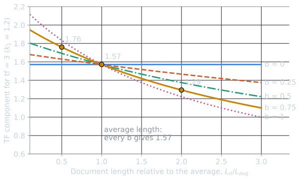
Why not always normalize fully? Long documents are long for two different reasons. Some are verbose, saying the same thing at greater length, and those should be normalized. Others have broader scope, covering more topics, and in those a high term count is real evidence. Partial normalization, with $b$ near 0.75, is a compromise that works well across typical collections. Where most length variation is verbosity, a higher $b$ helps.
The IDF component
BM25 inherits its IDF from the BIM's weight in the case with no relevance information:
$$\mathrm{IDF}(t) = \log \frac{N - \mathrm{df}_t + 0.5}{\mathrm{df}_t + 0.5}$$
where $N$ is the number of documents and $\mathrm{df}_t$ the number containing $t$. As in the BIM, this is negative for terms in more than half of the collection, which can make adding a common word to a query lower the score of documents that contain it. Lucene avoids this by adding 1 inside the logarithm:
$$\mathrm{IDF}_{\text{Lucene}}(t) = \log \left(1 + \frac{N - \mathrm{df}_t + 0.5}{\mathrm{df}_t + 0.5}\right)$$
In a collection of 1,000 documents, a term in 600 of them gets $-0.41$ under the first form and $0.51$ under Lucene's. For rare terms the two are nearly identical (4.55 and 4.56 for a term in 10 documents). The BIM article plots the forms side by side. When relevance judgments are available, the IDF can be replaced by the full Robertson–Spärck Jones weight from the BIM, which is how BM25 incorporates relevance feedback.
Long queries
The original formulation also saturates term frequency in the query, with a third parameter $k_3$:
$$\frac{(k_3 + 1)\,\mathrm{tf}_{t,q}}{k_3 + \mathrm{tf}_{t,q}}$$
For short keyword queries, where each term appears once, this factor is 1 and is usually omitted. It matters when the "query" is a paragraph or a whole document, as in finding similar documents. Even there, Robertson and Walker (1994) found that a very large $k_3$, which makes the factor linear in query term frequency, worked best, and Robertson and Zaragoza (2009) summarize the experiments as showing that saturation in the query is unimportant. Many implementations therefore simply count a repeated query term again.
A worked score: Cranfield query 185
The BIM article scores Cranfield query 185, experimental studies on panel flutter, and finds that all nine relevant abstracts share the top 20 places with eleven others, in large groups of tied scores. BM25 breaks those ties with term counts and lengths. The numbers below come from tools/experiments/cranfield/bm25_example.py, with Lucene's IDF in natural logs, $k_1 = 1.2$, $b = 0.75$, and lengths counted in tokens after stopping. The 1,400 abstracts average $L_{\mathrm{avg}} = 111.65$ tokens.
| Term | $\mathrm{df}_t$ | $\mathrm{IDF}(t) = \ln\left(1 + \frac{1400 - \mathrm{df}_t + 0.5}{\mathrm{df}_t + 0.5}\right)$ |
|---|---|---|
| experiment | 339 | 1.4175 |
| studi | 240 | 1.7622 |
| panel | 45 | 3.4272 |
| flutter | 56 | 3.2107 |
The six highest-scoring abstracts, with the length factor of each:
| Rank | Abstract | Judged | Length $L_d$ | $L_d / L_{\mathrm{avg}}$ | $K = 1.2\,(0.25 + 0.75\, L_d / L_{\mathrm{avg}})$ |
|---|---|---|---|---|---|
| 1 | 856 | relevant | 172 | 1.541 | 1.6865 |
| 2 | 857 | relevant | 175 | 1.567 | 1.7107 |
| 3 | 766 | relevant | 192 | 1.720 | 1.8477 |
| 4 | 390 | not relevant | 90 | 0.806 | 1.0255 |
| 5 | 858 | relevant | 149 | 1.335 | 1.5011 |
| 6 | 1008 | relevant | 58 | 0.519 | 0.7675 |
Each term's contribution is $\mathrm{IDF}(t) \times \frac{2.2\, \mathrm{tf}}{\mathrm{tf} + K}$, shown as "tf: contribution":
| Abstract | experiment | studi | panel | flutter | Score |
|---|---|---|---|---|---|
| 856 | 4: 2.194 | 5: 2.899 | 16: 6.821 | 11: 6.125 | 18.038 |
| 857 | 3: 1.986 | 2: 2.090 | 16: 6.812 | 7: 5.676 | 16.564 |
| 766 | 4: 2.133 | 0: 0 | 14: 6.661 | 10: 5.962 | 14.756 |
| 390 | 0: 0 | 2: 2.563 | 5: 6.257 | 5: 5.861 | 14.681 |
| 858 | 3: 2.079 | 0: 0 | 11: 6.635 | 7: 5.816 | 14.529 |
| 1008 | 1: 1.764 | 0: 0 | 6: 6.685 | 4: 5.926 | 14.375 |
One row by hand, for abstract 1008, the shortest: $K = 1.2 \times (0.25 + 0.75 \times 58 / 111.65) = 0.7675$. For panel, $\frac{2.2 \times 6}{6 + 0.7675} = 1.9505$, times 3.4272 gives 6.685. For flutter, $\frac{2.2 \times 4}{4 + 0.7675} = 1.8458$, times 3.2107 gives 5.926. For experiment, $\frac{2.2 \times 1}{1 + 0.7675} = 1.2447$, times 1.4175 gives 1.764. The sum is 14.375.
The table shows each mechanism at work.
- Saturation flattens the rare terms. Panel contributes between 6.26 and 6.82 to every one of these abstracts, whether it occurs 5 times or 16. Its maximum possible contribution is $2.2 \times 3.4272 = 7.54$, and all six are close to it. Once the rare terms are saturated, the ranking among these abstracts is decided by the common terms experiment and studi, as in the BIM, but now with graded contributions.
- Length normalization rescues short documents. Abstract 1008, at half the average length, reaches 1.95 of a possible 2.2 for panel from six occurrences, while abstract 766, at 1.7 times the average, needs fourteen occurrences for 1.94.
- Lexical evidence has limits. Abstract 390, some panel-flutter studies using piston theory, ranks fourth. It is a theoretical study, so it is not relevant to a request for experiments, but it uses three of the four query words at a short length. No weighting of terms can see that it lacks what experimental asked for, beyond the absence of one word.
Across all 542 abstracts that contain a query term, the nine relevant ones land at ranks 1, 2, 3, 5, 6, 9, 12, 14, and 15, for an average precision of 0.784, against 0.659 for the BIM without judgments. Setting $k_1 = 0$ turns BM25 back into the BIM with Lucene's IDF, and the average precision returns to exactly 0.659.
Try it
The demo scores the same 542 abstracts. Moving $k_1$ reshapes the term frequency curve, moving $b$ separates the curves for short and long documents, and the table shows how the top ten respond.
Some things to try: press Binary and watch the curve flatten to the BIM's step and the ranking collapse into ties broken by document number; press No length norm. and see the three curves merge while the short abstracts 1008 and 864 drop (from 6th to 8th and from 8th to 13th) and the long relevant abstract 859 rises from 9th to 7th; raise $k_1$ toward 3 and see abstracts with many occurrences pull ahead. For this one query the average precision moves between 0.659 (at $k_1 = 0$) and 0.829 (near $k_1 = 2.5$, $b = 0.7$) over the slider range. A single query is far too little to tune on, and comparing ranking models tunes the two parameters properly over held-out queries.
Tuning
Manning, Raghavan, and Schütze suggest $k_1$ (and $k_3$) between 1.2 and 2 and $b = 0.75$ when there is no data to tune on. Lucene's defaults are $k_1 = 1.2$ and $b = 0.75$. With a set of queries and relevance judgments, both parameters can be fitted by grid search against a measure such as MAP or nDCG. The best values depend on the collection: short, uniform documents such as product titles or tweets are less sensitive to $b$, and collections of long, verbose documents usually favor stronger normalization.
Variants
- BM25F handles documents with fields such as title, body, and anchor text. It combines weighted term frequencies across fields first and saturates once, instead of adding separate per-field scores.
- BM25L and BM25+ (Lv and Zhai, 2011a, 2011b) address a bias against very long documents. With strong length normalization, a term in a long document can contribute almost nothing, so a long relevant document may score below a short one that lacks the term. BM25+ adds a small constant lower bound to the contribution of any term that occurs at all.
Common misreadings
- "$k_1$ is the maximum contribution." The maximum of the term frequency component is $k_1 + 1$, and the term's maximum contribution is $(k_1 + 1)\,\mathrm{IDF}(t)$. $k_1$ is better read as the count at which a term in an average-length document earns half of that.
- "$b = 1$ divides by length." Full normalization divides the count by the relative length before saturating, so a document twice as long needs twice the occurrences for the same score. It does not divide the score by length.
- "BM25 scores are probabilities." The derivation dropped every constant that would make them so, as the BIM's did. Scores order documents for one query and are not comparable across queries.
Why it still matters
BM25 has no learned parameters beyond $k_1$ and $b$, needs no training data, indexes quickly, and explains its scores term by term. On the Cranfield collection, with default parameters, it reaches the highest mean average precision of the classical models compared in comparing ranking models, and implementing BM25 gives a tested implementation. Neural retrievers outperform it on the collections they were trained on, but the BEIR benchmark (Thakur and colleagues, 2021) showed that across a varied set of unseen domains BM25 remained competitive with the neural retrievers of the time, and better on several collections. Production systems therefore commonly combine the two: BM25 retrieves a candidate set cheaply, and a neural model re-ranks it, or the two rankings are fused in hybrid search. Retrieval-augmented generation systems use the same pattern to find passages for a language model.
BM25 also embodies the gap the Probability Ranking Principle leaves open. Its scores are not probabilities, but they track the probability of relevance closely enough, across enough collections, that the ordering they produce is very hard to beat without training data.
References
- Lv, Y., and Zhai, C. (2011a). When documents are very long, BM25 fails! In Proceedings of SIGIR 2011, 1103–1104.
- Lv, Y., and Zhai, C. (2011b). Lower-bounding term frequency normalization. In Proceedings of CIKM 2011, 7–16.
- Manning, C. D., Raghavan, P., and Schütze, H. (2008). Introduction to Information Retrieval, section 11.4.3. Cambridge University Press.
- Robertson, S. E., and Walker, S. (1994). Some simple effective approximations to the 2-Poisson model for probabilistic weighted retrieval. In Proceedings of SIGIR 1994, 232–241.
- Robertson, S. E., Walker, S., Jones, S., Hancock-Beaulieu, M., and Gatford, M. (1995). Okapi at TREC-3. In Overview of the Third Text REtrieval Conference (TREC-3), NIST Special Publication 500-225, 109–126.
- Robertson, S., and Zaragoza, H. (2009). The probabilistic relevance framework: BM25 and beyond. Foundations and Trends in Information Retrieval, 3(4), 333–389.
- Thakur, N., Reimers, N., Rücklé, A., Srivastava, A., and Gurevych, I. (2021). BEIR: A heterogeneous benchmark for zero-shot evaluation of information retrieval models. In Proceedings of the NeurIPS 2021 Datasets and Benchmarks Track.