The Binary Independence Model (BIM) is the classic probabilistic model of retrieval, developed by Stephen Robertson and Karen Spärck Jones (1976). It takes the Probability Ranking Principle literally: rank documents by $P(R = 1 \mid d, q)$. Two simplifying assumptions, given in its name, make that probability computable. The result is a ranking function that is a plain sum of term weights, and in the special case where nothing is known about relevance, those weights become inverse document frequency. That connection matters because it gives a probabilistic justification for a heuristic widely used in practice.
This article derives the model step by step, then carries one real query through it: Cranfield query 185, experimental studies on panel flutter, over the 1,400 abstracts of the Cranfield collection, which has relevance judgments for every query. The numbers are computed by tools/experiments/cranfield/bim_example.py, with natural logarithms, and rounded as shown. The probability primer reviews Bayes' rule, odds, and smoothing.
Assumptions
Binary. A document is represented only by which vocabulary terms it contains. Over a vocabulary of $M$ terms, document $d$ becomes a vector $\vec{x} = (x_1, \dots, x_M)$ with $x_t = 1$ if term $t$ occurs in $d$ and $x_t = 0$ otherwise. How often a term occurs, where it occurs, and how long the document is are all discarded. The query is represented the same way, as a vector $\vec{q}$.
Independence. Given the relevance class, terms occur independently of one another:
$$P(\vec{x} \mid R, q) = \prod_{t=1}^{M} P(x_t \mid R, q).$$
This is the same conditional independence assumption that underlies Naive Bayes classification, and it is false in the same way. "Hong" and "Kong" are not independent. Like Naive Bayes, the BIM often ranks well anyway, because a ranking needs only the order of the scores to be right, not the probabilities themselves.
A third assumption is easy to overlook: terms that do not appear in the query are distributed identically in relevant and nonrelevant documents, so they cannot affect the ranking.
What the model can see
The binary assumption has a concrete consequence worth seeing before any algebra. Query 185 has four terms after stemming and stopping: experiment, studi, panel, and flutter. Under the third assumption, only these four matter, so the BIM sees each document as one of $2^4 = 16$ presence-absence patterns. Every document with the same pattern receives the same score. The 1,400 Cranfield abstracts fall into 15 of the 16 patterns (one, studi and flutter without the other two, is empty), and 858 of them contain none of the four terms. Whatever weights the model assigns, all it can do is put these 15 groups in some order. The rest of the derivation decides which order.
Deriving the ranking function
The derivation follows Manning, Raghavan, and Schütze (2008, §11.3.1). Each step either uses a rule of probability or discards something that is the same for every document and so cannot change the ranking.
Step 1. Bayes' rule. Start from the quantity the PRP says to rank by and turn it around, so that it is expressed through how documents look in each relevance class:
$$P(R = 1 \mid \vec{x}, \vec{q}) = \frac{P(\vec{x} \mid R = 1, \vec{q}) \, P(R = 1 \mid \vec{q})}{P(\vec{x} \mid \vec{q})}.$$
Step 2. Rank by odds. The denominator $P(\vec{x} \mid \vec{q})$, the probability of seeing exactly this document vector, is hard to estimate. It disappears if we rank by the odds of relevance instead, which are monotonic in the probability and so give the same ordering. Writing Bayes' rule for $R = 0$ as well and dividing, the denominators cancel:
$$O(R \mid \vec{x}, \vec{q}) = \frac{P(R = 1 \mid \vec{x}, \vec{q})}{P(R = 0 \mid \vec{x}, \vec{q})} = \underbrace{\frac{P(R = 1 \mid \vec{q})}{P(R = 0 \mid \vec{q})}}_{O(R \mid \vec{q})} \cdot \frac{P(\vec{x} \mid R = 1, \vec{q})}{P(\vec{x} \mid R = 0, \vec{q})}.$$
The prior odds $O(R \mid \vec{q})$ are the same for every document, so they do not affect the ranking.
Step 3. Independence. The remaining ratio compares the probability of a whole vector in the two classes, which would need an estimate for each of $2^M$ vectors. The independence assumption factors it into one ratio per term:
$$O(R \mid \vec{x}, \vec{q}) = O(R \mid \vec{q}) \cdot \prod_{t=1}^{M} \frac{P(x_t \mid R = 1, \vec{q})}{P(x_t \mid R = 0, \vec{q})}.$$
Step 4. Name the two probabilities per term. Each $x_t$ is 0 or 1, so each term needs only two numbers:
- $p_t = P(x_t = 1 \mid R = 1, \vec{q})$, the probability that term $t$ appears in a relevant document.
- $u_t = P(x_t = 1 \mid R = 0, \vec{q})$, the probability that it appears in a nonrelevant document.
A present term contributes the ratio $p_t / u_t$, and an absent term contributes $(1 - p_t)/(1 - u_t)$.
Step 5. Drop the terms not in the query. Assuming $p_t = u_t$ for terms not in the query, those terms contribute a factor of 1 whether present or absent. For query terms, split the product by whether the term is present in the document:
$$O(R \mid \vec{x}, \vec{q}) = O(R \mid \vec{q}) \cdot \prod_{t:\, x_t = q_t = 1} \frac{p_t}{u_t} \cdot \prod_{t:\, x_t = 0,\, q_t = 1} \frac{1 - p_t}{1 - u_t}.$$
Step 6. Move the absent terms into a constant. The second product runs over query terms the document lacks, which is awkward to compute because it depends on what is missing. Multiply and divide by $\frac{1 - p_t}{1 - u_t}$ for the query terms the document does contain. The multiplied copies complete the second product so that it runs over all query terms, and the divided copies join the first product:
$$O(R \mid \vec{x}, \vec{q}) = O(R \mid \vec{q}) \cdot \prod_{t:\, x_t = q_t = 1} \frac{p_t (1 - u_t)}{u_t (1 - p_t)} \cdot \prod_{t:\, q_t = 1} \frac{1 - p_t}{1 - u_t}.$$
The last product depends only on the query, so it is constant across documents and can be dropped along with the prior odds. The absent terms have not been ignored: their evidence has been folded into the weight of the present ones, because each present term's factor now records both "present rather than absent in a relevant document" and "present rather than absent in a nonrelevant one".
Step 7. Take logarithms. The logarithm preserves order and turns the product into a sum, giving the retrieval status value:
$$\mathrm{RSV}_d = \sum_{t:\, x_t = q_t = 1} c_t, \qquad c_t = \log \frac{p_t (1 - u_t)}{u_t (1 - p_t)} = \log \frac{p_t}{1 - p_t} + \log \frac{1 - u_t}{u_t}.$$
Each matching query term adds a fixed weight $c_t$. The weight is a log odds ratio: the log odds of the term appearing in a relevant document, minus the log odds of it appearing in a nonrelevant one. A term that appears much more often in relevant documents gets a large positive weight, a term that appears equally often in both gets a weight near zero, and a term that is more common in nonrelevant documents gets a negative weight. Because the score is a sum over terms the document contains, it can be computed directly from the postings lists of an inverted index, visiting only documents that contain at least one query term.
The RSV is not a probability, and nothing in steps 2, 6, and 7 tried to keep it one. Three quantities were dropped or transformed (the prior odds, the product over all query terms, and the scale through the logarithm), each harmless for ranking and fatal for calibration.
Estimating the term weights
With relevance judgments
Suppose that for a query we know which documents are relevant. For each query term, a contingency table summarizes the collection:
| Relevant | Nonrelevant | Total | |
|---|---|---|---|
| Term present ($x_t = 1$) | $s$ | $\mathrm{df}_t - s$ | $\mathrm{df}_t$ |
| Term absent ($x_t = 0$) | $S - s$ | $(N - \mathrm{df}_t) - (S - s)$ | $N - \mathrm{df}_t$ |
| Total | $S$ | $N - S$ | $N$ |
Here $N$ is the collection size, $S$ the number of relevant documents, $\mathrm{df}_t$ the number of documents containing $t$, and $s$ the number of relevant documents containing $t$. The maximum likelihood estimates are $p_t = s/S$ and $u_t = (\mathrm{df}_t - s)/(N - S)$. These break down whenever a cell is zero, for example a term that appears in every relevant document makes $1 - p_t = 0$. The standard fix adds $\tfrac{1}{2}$ to each cell, giving the Robertson–Spärck Jones weight:
$$c_t = \log \frac{(s + \tfrac12) \,/\, (S - s + \tfrac12)}{(\mathrm{df}_t - s + \tfrac12) \,/\, (N - \mathrm{df}_t - S + s + \tfrac12)}.$$
The numerator is the smoothed odds $p_t / (1 - p_t)$ with $p_t = (s + \tfrac12)/(S + 1)$, and the denominator is the smoothed odds $u_t / (1 - u_t)$ with $u_t = (\mathrm{df}_t - s + \tfrac12)/(N - S + 1)$, so the weight is still the log odds ratio of step 7, computed from smoothed estimates.
Worked example. A collection has $N = 1000$ documents, and for the query tropical fish we know $S = 10$ are relevant. Using natural logarithms:
| Term | $\mathrm{df}_t$ | $s$ | $p_t$ | $u_t$ | $c_t$ with judgments | $c_t$ without |
|---|---|---|---|---|---|---|
| tropical | 50 | 8 | 0.80 | 0.042 | 4.33 | 2.94 |
| fish | 200 | 9 | 0.90 | 0.193 | 3.28 | 1.38 |
Without relevance information, fish looks like a weak term because it appears in a fifth of the collection. The judgments show it appears in nine of the ten relevant documents, and its weight more than doubles. This is exactly the evidence relevance feedback supplies.
A real query: Cranfield query 185
Query 185 has $S = 9$ relevant abstracts among $N = 1400$. The four contingency tables, written as one row per term with the four cells in the order of the table above:
| Term | $\mathrm{df}_t$ | Relevant, present ($s$) | Nonrelevant, present | Relevant, absent | Nonrelevant, absent |
|---|---|---|---|---|---|
| experiment | 339 | 5 | 334 | 4 | 1,057 |
| studi | 240 | 2 | 238 | 7 | 1,153 |
| panel | 45 | 9 | 36 | 0 | 1,355 |
| flutter | 56 | 9 | 47 | 0 | 1,344 |
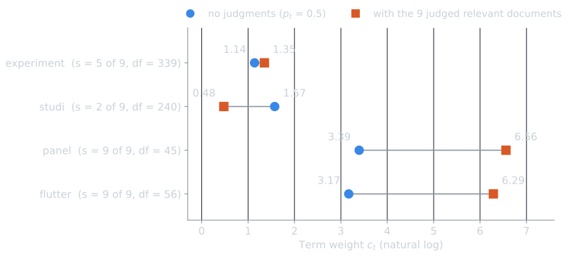
Every relevant abstract contains both panel and flutter, so for those two terms the maximum likelihood estimate is $p_t = 9/9 = 1$ and the unsmoothed weight is infinite. Smoothing gives $p_t = 9.5/10 = 0.95$. The estimates and the two halves of each weight:
| Term | $p_t$ | $u_t$ | $\log \frac{p_t}{1 - p_t}$ | $\log \frac{1 - u_t}{u_t}$ | $c_t$ with judgments | $c_t$ without |
|---|---|---|---|---|---|---|
| experiment | 0.550 | 0.240 | 0.201 | 1.151 | 1.352 | 1.140 |
| studi | 0.250 | 0.171 | −1.099 | 1.576 | 0.478 | 1.574 |
| panel | 0.950 | 0.026 | 2.944 | 3.615 | 6.559 | 3.394 |
| flutter | 0.950 | 0.034 | 2.944 | 3.343 | 6.287 | 3.170 |
The second half of each weight, $\log \frac{1 - u_t}{u_t}$, changes little when judgments are added (by at most 0.22, for panel), because removing 9 relevant documents from 1,400 hardly alters the nonrelevant statistics. The judgments act mainly through the first half, which is 0 without judgments. It contributes 2.94 to panel and flutter, since the judgments show they are close to necessary, and each of their weights rises by 3.1 to 3.2 in all. Studi loses 1.1: it appears in only 2 of the 9 relevant abstracts, a lower rate than its 0.5 default assumes, and its log odds in relevant documents turn negative.
Now the 15 groups of documents can be ordered. The table lists each presence pattern in the order the no-judgment weights rank it, with the number of abstracts that have the pattern and how many of them are relevant:
| Query terms present | Abstracts | Relevant | RSV without judgments | RSV with judgments |
|---|---|---|---|---|
| experiment, studi, panel, flutter | 2 | 2 | 9.28 | 14.68 |
| studi, panel, flutter | 2 | 0 | 8.14 | 13.32 |
| experiment, panel, flutter | 4 | 3 | 7.70 | 14.20 |
| panel, flutter | 12 | 4 | 6.56 | 12.85 |
| experiment, studi, panel | 3 | 0 | 6.11 | 8.39 |
| experiment, studi, flutter | 4 | 0 | 5.88 | 8.12 |
| studi, panel | 4 | 0 | 4.97 | 7.04 |
| experiment, panel | 6 | 0 | 4.53 | 7.91 |
| experiment, flutter | 12 | 0 | 4.31 | 7.64 |
| panel | 12 | 0 | 3.39 | 6.56 |
| flutter | 20 | 0 | 3.17 | 6.29 |
| experiment, studi | 72 | 0 | 2.71 | 1.83 |
| studi | 153 | 0 | 1.57 | 0.48 |
| experiment | 236 | 0 | 1.14 | 1.35 |
| none | 858 | 0 | 0.00 | 0.00 |
Several things are visible here that the formulas alone do not show.
- All nine relevant abstracts are in the top four groups, the twenty abstracts containing both panel and flutter. Even without judgments the model puts them in the top 20 of 542 candidates, because the two rare terms dominate the score.
- Within the top 20, the order is decided by the common terms. Without judgments, studi outweighs experiment (1.57 against 1.14, because it is rarer), so the two "studies on panel flutter" abstracts, neither relevant, rank above the four "experiment panel flutter" abstracts, three of them relevant. The judgments reverse those weights (0.48 against 1.35) and swap the two groups.
- Ties are large. The fourth group holds 12 abstracts with identical scores, four of them relevant. The BIM cannot separate an abstract that mentions flutter once in passing from one devoted to it. Breaking ties by document number, the relevant abstracts land at ranks 1, 2, 6, 7, 8, 10, 11, 16, 18 without judgments (average precision 0.659) and 1, 2, 4, 5, 6, 10, 11, 16, 18 with them (0.736). Term frequency is exactly the information that would break these ties, which is what BM25 adds; on the same query it reaches 0.784.
Using a query's own judgments to score that same query, as here, shows what the weights mean but overstates what feedback achieves, since the judged documents are counted in the evaluation. The fair version, which evaluates only on documents the user has not judged, is in relevance feedback.
Without relevance judgments
At query time there are usually no judgments at all. Two approximations recover a usable model.
- Nonrelevant documents look like the collection. Relevant documents are a tiny fraction of most collections, so the term statistics of nonrelevant documents are close to those of the collection as a whole: $u_t \approx \mathrm{df}_t / N$. The query 185 table shows how good this is: the judged $u_t$ for panel is 0.026, and $\mathrm{df}_t / N = 45/1400 = 0.032$.
- A neutral guess for $p_t$. With no evidence about relevant documents, Croft and Harper (1979) assumed that $p_t$ is the same for every query term. The usual choice is $p_t = 0.5$, which makes $\log \frac{p_t}{1 - p_t} = 0$.
The weight then reduces to
$$c_t = \log \frac{1 - u_t}{u_t} = \log \frac{N - \mathrm{df}_t}{\mathrm{df}_t} \approx \log \frac{N}{\mathrm{df}_t},$$
which is inverse document frequency. The heuristic weight of TF-IDF falls out of a probabilistic derivation as the special case of knowing nothing about relevance. The column "without" in the tables above uses the smoothed form, which is what the Robertson–Spärck Jones weight gives with $S = s = 0$: $\log \frac{N - \mathrm{df}_t + 0.5}{\mathrm{df}_t + 0.5}$ (Manning, Raghavan, and Schütze, 2008, eq. 11.31).
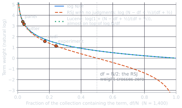
The exact form $\log \frac{N - \mathrm{df}_t}{\mathrm{df}_t}$ has a property the approximation hides: it is negative for any term that appears in more than half the collection. Under the model, a document containing such a term is slightly less likely to be relevant. That follows from the $p_t = 0.5$ assumption: a term in 70 percent of all documents but assumed to be in only 50 percent of relevant ones is evidence against relevance. Implementations usually either remove those terms as stopwords or switch to a variant that is always positive, a choice that resurfaces in BM25.
The $p_t = 0.5$ guess is the weak point of the no-judgment model, and query 185 shows it both ways: it underrates panel and flutter, which real relevant documents nearly always contain, and overrates studi. Manning, Raghavan, and Schütze (2008, §11.3.3) note an alternative proposed by Greiff, letting $p_t$ rise with $\mathrm{df}_t / N$, since common terms are also more likely to appear in relevant documents.
Between the two
Between full judgments and none, the model can bootstrap its own evidence by assuming the top-ranked documents are relevant and re-estimating $p_t$ from them. That is pseudo-relevance feedback. Using judgments from a real user is relevance feedback, which on the Cranfield collection raised the BIM's effectiveness on the documents the user had not yet seen by nearly half.
Common misreadings
- "The BIM is TF-IDF with binary term frequency." The two share an IDF-like weight only in the no-judgment case. The BIM's weight is a log odds ratio that changes with relevance information, and its derivation says how; TF-IDF has no such mechanism.
- "Absent query terms are ignored." Their evidence is folded into the weights of the present terms in step 6. A document lacking panel loses the 3.39 that panel would have added, which is the same as being penalized for its absence relative to one that has it.
- "The RSV is the log odds of relevance." It is the log odds up to two dropped constants, the prior odds and the product over all query terms, so it differs from the true log odds by an unknown amount that depends on the query. Scores can be compared across documents for one query, not across queries.
In practice
My implementation for CSC 790 (HW04 on GitHub) uses the no-judgment form: $p_t = 0.5$ and a smoothed $u_t = (\mathrm{df}_t + 0.5)/(N + 1)$, which makes each term's weight $\log_{10} \frac{N - \mathrm{df}_t + 0.5}{\mathrm{df}_t + 0.5}$. The program collects every document that appears in at least one query term's postings and computes a score for each. Three details are worth noting for anyone reusing the code:
- Negative weights. As described above, any term in more than half the collection gets a negative weight. A stop list removes most such terms, but not all.
- Unused judgments. The assignment supplied relevance labels for each query's documents. The program loads them only to print beside each result. Feeding them into the Robertson–Spärck Jones weight above would turn the same code into relevance feedback.
- Comment labels. The code's comments describe $p_t$ as the probability of the term "in the collection" and $u_t$ as the probability "in the document". In the model they are the probabilities of the term in relevant and nonrelevant documents, respectively.
The same model later served as the search engine in the Goodreads project, where it answered single queries over an index of 1,260,776 book reviews and 540,135 distinct terms in about 1.8 seconds on one machine, in Python.
Strengths and limitations
The BIM has a clear derivation in which every assumption is stated, and it shows that IDF has a probabilistic meaning. It can use relevance information when it has some and degrade gracefully when it has none.
Its weaknesses come straight from the binary representation. A document that mentions fish forty times scores the same as one that mentions it once in passing, and a long document has more chances to contain any given term, which the model does nothing to correct. The large tie groups of query 185 are the same weakness seen from the inside. In experiments on the TREC-2 ad hoc topics, binary weights reached an average precision of 0.199, against 0.300 once term frequency and document length were added (Robertson and Walker, 1994). The same happens on the Cranfield collection: without relevance information, the BIM reaches a mean average precision of 0.220, against 0.294 for TF-IDF and 0.307 for BM25 (see comparing ranking models). Fixing those two weaknesses within the probabilistic framework is what produced Okapi BM25.
References
- Croft, W. B., and Harper, D. J. (1979). Using probabilistic models of document retrieval without relevance information. Journal of Documentation, 35(4), 285–295.
- Manning, C. D., Raghavan, P., and Schütze, H. (2008). Introduction to Information Retrieval, sections 11.3–11.4. Cambridge University Press.
- Robertson, S. E., and Spärck Jones, K. (1976). Relevance weighting of search terms. Journal of the American Society for Information Science, 27(3), 129–146.
- Robertson, S. E., and Walker, S. (1994). Some simple effective approximations to the 2-Poisson model for probabilistic weighted retrieval. In Proceedings of SIGIR 1994, 232–241.