Naive Bayes needs a model of how a class generates a document, and there are two natural choices. The multinomial model treats a document as a sequence of words drawn one at a time from the class's distribution over the vocabulary, so repeated words count repeatedly. The Bernoulli model treats a document as the outcome of one coin flip per vocabulary term, heads if the term appears and tails if not, so it records which terms are present and also which are absent. The two can classify the same document differently, and they behave differently as the vocabulary grows. This article describes the Bernoulli model, works the textbook's example through it, compares the two models on Reuters, and then takes up a broader question: why a classifier based on an assumption known to be false works as well as it does.
The Bernoulli model
The generative story differs from the multinomial one in what is drawn (Manning, Raghavan, and Schütze, 2008, §13.3–13.4). To write a document of class $c$, go through the vocabulary once. For each term $t$, flip a coin that comes up heads with probability $P(t \mid c)$, and include $t$ in the document if it does. The document is the set of terms that came up heads. How many times a term occurs, and in what order, is not part of the model.
For each class $c$ and each term $t$ in the vocabulary $V$, the model therefore has a parameter $P(t \mid c)$, the probability that a document of class $c$ contains $t$ at least once. A document's probability given the class multiplies over the whole vocabulary, one factor per coin:
$$P(d \mid c) = \prod_{t \in V} \begin{cases} P(t \mid c) & \text{if } t \in d, \\ 1 - P(t \mid c) & \text{if } t \notin d. \end{cases}$$
The parameters are estimated from document counts, smoothed by adding one to each of the two outcomes:
$$\hat{P}(t \mid c) = \frac{N_{ct} + 1}{N_c + 2},$$
where $N_{ct}$ is the number of training documents of class $c$ that contain $t$ and $N_c$ the number of training documents of class $c$. The maximum likelihood estimate, without the added counts, is the fraction $N_{ct}/N_c$ of the class's documents that contain the term; the derivation is the one for the multinomial model with two outcomes per coin instead of $\lvert V \rvert$ outcomes per token. This is the same document representation as the Binary Independence Model, whose probabilities $p_t$ and $u_t$ are Bernoulli parameters for the relevant and nonrelevant classes. The section on the linear form below shows that the connection is exact.
Where the two models disagree
The worked example of Naive Bayes classification has three training documents of class China (Chinese Beijing Chinese, Chinese Chinese Shanghai, Chinese Macao) and one of class Japan (Tokyo Japan Chinese), and the test document Chinese Chinese Chinese Tokyo Japan. The multinomial model chose China. The Bernoulli model counts documents, not tokens. Chinese occurs five times in the China documents but in only three documents, so $N_{ct} = 3$. The estimates $(N_{ct} + 1)/(N_c + 2)$, with $N_c = 3$ for China and $N_c = 1$ for Japan (Manning, Raghavan, and Schütze, 2008, §13.3):
| Term | China: $N_{ct}$ and estimate | Japan: $N_{ct}$ and estimate | In test? |
|---|---|---|---|
| Chinese | 3, 4/5 = 0.8 | 1, 2/3 | yes |
| Japan | 0, 1/5 = 0.2 | 1, 2/3 | yes |
| Tokyo | 0, 1/5 = 0.2 | 1, 2/3 | yes |
| Beijing | 1, 2/5 = 0.4 | 0, 1/3 | no |
| Macao | 1, 2/5 = 0.4 | 0, 1/3 | no |
| Shanghai | 1, 2/5 = 0.4 | 0, 1/3 | no |
$$\hat{P}(\textit{China} \mid d) \propto \tfrac{3}{4} \times 0.8 \times 0.2 \times 0.2 \times (1 - 0.4)^3 \approx 0.005,$$
$$\hat{P}(\textit{Japan} \mid d) \propto \tfrac{1}{4} \times \left(\tfrac{2}{3}\right)^3 \times \left(1 - \tfrac{1}{3}\right)^3 \approx 0.022.$$
The Bernoulli model chooses Japan. The same calculation in natural logarithms, one row per coin, shows where the decision comes from (computed by tools/experiments/reuters/china_japan.py, rounded to three decimals):
| Factor | China | Japan | Difference, China − Japan |
|---|---|---|---|
| Prior | log 0.75 = −0.288 | log 0.25 = −1.386 | +1.099 |
| Chinese present | log 0.8 = −0.223 | log 2/3 = −0.405 | +0.182 |
| Tokyo present | log 0.2 = −1.609 | −0.405 | −1.204 |
| Japan present | −1.609 | −0.405 | −1.204 |
| Beijing absent | log 0.6 = −0.511 | log 2/3 = −0.405 | −0.105 |
| Macao absent | −0.511 | −0.405 | −0.105 |
| Shanghai absent | −0.511 | −0.405 | −0.105 |
| Total | −5.262 | −3.819 | −1.443 |
The log odds are −1.443, and normalizing the two scores gives $\hat{P}(\textit{China} \mid d) = 0.191$, against 0.690 under the multinomial model. The decisive difference is that the Bernoulli model counts Chinese once. In the multinomial model its three occurrences multiplied the odds for China by $(27/14)^3 \approx 7.2$; here its single presence multiplies them only by $0.8/(2/3) = 1.2$, a log contribution of 0.182, far too little to offset Japan and Tokyo. Those two are present in the one Japan document but in none of the China documents, and each costs China 1.204.
The model also counts absences: Beijing, Macao, and Shanghai each appear in China documents, so their absence from the test document counts against China, 0.105 each. The decision would be Japan even without them. Leaving out the absent terms, the scores are 0.024 for China and 0.074 for Japan. Which answer is right depends on whether repetition and absence carry information in the collection at hand.
The linear form, and the BIM's term weights
Like the multinomial model, the Bernoulli model is a linear classifier, and writing it that way connects it to retrieval. Let $x_t = 1$ if term $t$ is in the document and 0 otherwise, and write $p_t = \hat{P}(t \mid c)$ and $u_t = \hat{P}(t \mid \bar{c})$. Each coin's factor can be written without cases as $p_t^{x_t} (1 - p_t)^{1 - x_t}$, so
$$\log P(d \mid c) = \sum_{t \in V} \Big[ x_t \log p_t + (1 - x_t) \log (1 - p_t) \Big] = \sum_{t \in V} \log (1 - p_t) + \sum_{t \in V} x_t \log \frac{p_t}{1 - p_t}.$$
The first sum does not depend on the document. Subtracting the same expression for $\bar{c}$ and adding the prior ratio gives the log odds:
$$\log \frac{\hat{P}(c \mid d)}{\hat{P}(\bar{c} \mid d)} = \underbrace{\log \frac{\hat{P}(c)}{\hat{P}(\bar{c})} + \sum_{t \in V} \log \frac{1 - p_t}{1 - u_t}}_{\text{constant}} + \sum_{t \in d} \log \frac{p_t (1 - u_t)}{u_t (1 - p_t)}.$$
The weight on each present term, $\log \frac{p_t (1 - u_t)}{u_t (1 - p_t)}$, is exactly the term weight $c_t$ of the Binary Independence Model, with class $c$ in the role of "relevant". The BIM ranks documents by the sum of these weights over the query terms they contain, having assumed that terms outside the query are equally likely in relevant and nonrelevant documents, which makes their weights zero. Bernoulli Naive Bayes classifies by the sum over all vocabulary terms the document contains, plus a constant, compared with zero. The two are the same model put to different uses: one ranks, so it can drop the constant, and the other decides, so it cannot.
On the running example the constant is the prior's $\log 3 = 1.099$ plus $\sum_t \log \frac{1 - p_t}{1 - u_t}$ over all six terms: $-0.511$ for Chinese, $-0.105$ for each of the three cities, and $+0.875$ for each of Tokyo and Japan, so 2.023 in total. The presence weights are:
| Term | Presence weight $\log \frac{p_t(1 - u_t)}{u_t(1 - p_t)}$ |
|---|---|
| Chinese | 0.693 |
| Beijing, Macao, Shanghai | 0.288 |
| Tokyo, Japan | −2.079 |
The test document contains Chinese, Tokyo, and Japan, so its log odds are $2.023 + 0.693 - 2.079 - 2.079 = -1.443$ (summed before rounding), the same as the table above. The form also explains why the Bernoulli model suffers with large vocabularies. The constant holds a term for every word in the vocabulary, and every word a document lacks has, in effect, cast a vote.
Which model is better?
McCallum and Nigam (1998) compared the two on several text collections. The Bernoulli model performed well with small vocabularies, but its accuracy fell as the vocabulary grew. The multinomial model improved with larger vocabularies and was better overall. One reason is the absence terms. With a vocabulary of tens of thousands of terms, the product over absent terms dominates the Bernoulli score, and most of those absences are uninformative. Long documents also suffer, since a long document is likely to contain many terms that are rare in its class.
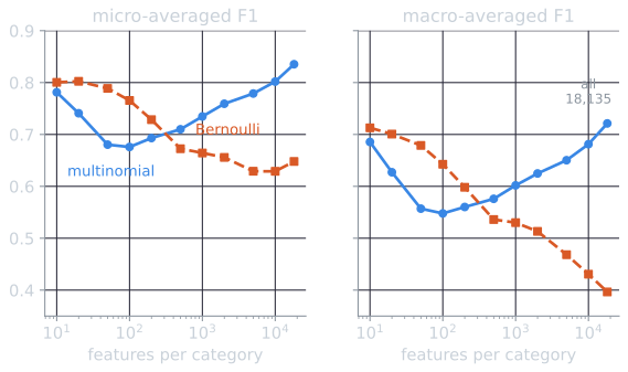
The Reuters experiments used throughout this topic show the same pattern. Both models were trained on the ten largest categories with the top $k$ terms per category selected by mutual information (see feature selection), for $k$ from 10 to all 18,135:
| Features per category | Bernoulli micro / macro F1 | Multinomial micro / macro F1 |
|---|---|---|
| 10 | 0.800 / 0.713 | 0.781 / 0.686 |
| 50 | 0.789 / 0.679 | 0.680 / 0.557 |
| 100 | 0.765 / 0.643 | 0.676 / 0.548 |
| 500 | 0.673 / 0.536 | 0.710 / 0.576 |
| 1,000 | 0.664 / 0.530 | 0.735 / 0.602 |
| 5,000 | 0.629 / 0.468 | 0.779 / 0.650 |
| All 18,135 | 0.648 / 0.396 | 0.835 / 0.721 |
The Bernoulli model does best with the smallest feature sets and degrades steadily as more are added. With up to about 200 features it beats the multinomial model with the same features, at 50 features by 0.789 against 0.680 micro-F1. But the multinomial model with all 18,135 features reaches 0.835 micro-F1 and 0.721 macro-F1, better than any Bernoulli setting on micro-F1. With features chosen by the χ² statistic instead, the Bernoulli model's best result is 0.817 micro-F1 and 0.729 macro-F1 at 10 features: slightly better than the full multinomial model on macro-F1, still worse on micro-F1. The Bernoulli model suits short documents and small, carefully chosen vocabularies, and the multinomial model suits everything else.
Why Naive Bayes works
Both models assume that terms occur independently given the class. For text this is badly wrong: words come in phrases, topics bring clusters of related words, and a document that mentions Hong almost certainly mentions Kong. Yet Naive Bayes is competitive with far more elaborate methods on many text tasks. The explanation lies in what classification requires.
Classification needs only the right winner. A classifier is correct if the true class receives the highest score. The scores need not be accurate probabilities. Domingos and Pazzani (1997) showed that Naive Bayes is optimal under zero-one loss, the loss that counts only whether the chosen class is correct, in many situations where the independence assumption is violated. Violations distort the estimated probabilities, often by large factors, but frequently not enough to change which class is largest.
Violations push toward the same answer. Correlated words that indicate a class are counted as independent evidence, so their contribution is counted more than once. When Hong and Kong both appear, a classifier that treats them as independent adds both weights, though the second word carries almost no new information. When the correlated words all point to the true class, the overcounting makes the classifier more confident without changing its decision.
The probabilities are poorly calibrated. The price of double counting is that Naive Bayes's probability estimates are extreme, usually very close to 0 or 1 (Manning, Raghavan, and Schütze, 2008, §13.4). A Naive Bayes classifier that reports 0.999 is not right 99.9 percent of the time. The Reuters experiments measure how far off it is. Each of the ten category classifiers produced a posterior probability for each of the 3,019 test stories, 30,190 probabilities in all. Grouping them by the probability reported and counting how many stories in each group actually belong to the category:
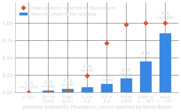
96.5 percent of the probabilities are below 0.001 or above 0.999. Of the 2,866 stories assigned a probability above $1 - 10^{-6}$, 85.5 percent belong to the category, and of the 314 assigned between 0.999 and $1 - 10^{-6}$, only 44.9 percent. A probability of 0.999 here means roughly a coin flip. The ranking is still useful: higher probabilities do mean more stories in the category, so the order of the scores carries information that the values themselves misstate. Where calibrated probabilities matter, as in setting a threshold that trades precision for recall, or combining a classifier's output with other evidence, the scores must be recalibrated or another method used. Evaluating classifiers shows that moving the threshold well above the nominal probability of 0.5 improves F1 substantially on these categories.
Simple models resist overfitting. With little training data, a model with few parameters, one probability per term per class and nothing for interactions between terms, cannot fit noise in those interactions. Naive Bayes therefore does relatively well on small training sets, which is common in practice.
Its weaknesses are also well understood. Rennie, Shih, Teevan, and Karger (2003) identified several systematic biases in multinomial Naive Bayes for text, such as favoring classes with more training data. They showed that simple corrections, including training on the complement of each class and transforming term frequencies, brought it close to support vector machines. On the Reuters categories here, a k-nearest-neighbor classifier with 10 or more neighbors does better, which is typical of comparisons between Naive Bayes and stronger methods.
References
- Domingos, P., and Pazzani, M. (1997). On the optimality of the simple Bayesian classifier under zero-one loss. Machine Learning, 29(2–3), 103–130.
- Manning, C. D., Raghavan, P., and Schütze, H. (2008). Introduction to Information Retrieval, sections 13.3–13.4. Cambridge University Press.
- McCallum, A., and Nigam, K. (1998). A comparison of event models for Naive Bayes text classification. In AAAI-98 Workshop on Learning for Text Categorization, 41–48.
- Rennie, J. D. M., Shih, L., Teevan, J., and Karger, D. R. (2003). Tackling the poor assumptions of Naive Bayes text classifiers. In Proceedings of ICML 2003, 616–623.