Naive Bayes classifies a document by asking which class would most probably have generated its words. A different approach asks which documents the new one most resembles. In the vector space model, every document is a weighted term vector, and cosine similarity measures how alike two documents are. If documents of the same class lie near one another in that space, a new document can be classified by where it falls. This is vector space classification. It reuses the representation built for retrieval rather than a probabilistic model of text. This article describes its two classic methods, Rocchio and k nearest neighbors, works both on a small example in two dimensions where their decision regions can be drawn, and compares them with Naive Bayes on Reuters.
The contiguity hypothesis
Vector space classifiers rest on the contiguity hypothesis: documents in the same class form a contiguous region of the space, and regions of different classes do not overlap (Manning, Raghavan, and Schütze, 2008, ch. 14). Whether it holds depends on the representation. With TF-IDF vectors, documents about grain share vocabulary such as wheat, tonnes, and harvest, and so cluster together. A class defined by something other than topic, such as the author's gender or a document's date, may not form a region at all, and no vector space classifier will learn it well.
Real document vectors have thousands of dimensions, which cannot be drawn. The geometry of the two methods is the same in any number of dimensions, so this article illustrates them in a plane. In the example below, each point is a training document of class A (circles) or class B (squares). Class A forms one cloud in the middle. Class B forms two clouds, one on each side, as a class made of two distinct subtopics would. The coordinates are in tools/experiments/reuters/toy2d.py, which computes every number quoted for the example.
Rocchio classification
Rocchio classification represents each class by its centroid, the average of the vectors of its training documents,
$$\vec{\mu}(c) = \frac{1}{\lvert D_c \rvert} \sum_{d \in D_c} \vec{v}(d),$$
where $D_c$ is the set of training documents in class $c$, and assigns a new document to the class whose centroid is nearest. It adapts the centroid computation of Rocchio relevance feedback to classification. Training is a single pass to compute the centroids, and classification needs one distance or similarity per class.
Its boundary is a hyperplane
For two classes A and B, a point $\vec{x}$ is assigned to A when it is closer to A's centroid:
$$\lVert \vec{x} - \vec{\mu}_A \rVert^2 < \lVert \vec{x} - \vec{\mu}_B \rVert^2.$$
Expanding both squared distances, $\lVert \vec{x} \rVert^2 - 2\, \vec{x} \cdot \vec{\mu} + \lVert \vec{\mu} \rVert^2$, the $\lVert \vec{x} \rVert^2$ terms cancel, leaving
$$2 (\vec{\mu}_A - \vec{\mu}_B) \cdot \vec{x} > \lVert \vec{\mu}_A \rVert^2 - \lVert \vec{\mu}_B \rVert^2.$$
This is a weight vector $\vec{w} = 2(\vec{\mu}_A - \vec{\mu}_B)$ and a threshold $b = \lVert \vec{\mu}_A \rVert^2 - \lVert \vec{\mu}_B \rVert^2$: a document goes to A when $\vec{w} \cdot \vec{x} > b$. The boundary $\vec{w} \cdot \vec{x} = b$ is the hyperplane that perpendicularly bisects the segment between the two centroids, so Rocchio is a linear classifier (Manning, Raghavan, and Schütze, 2008, §14.2). When documents are length-normalized and the centroids are length-normalized as well, as in the Reuters experiment below, the comparison of cosines $\vec{x} \cdot \hat{\mu}_A > \vec{x} \cdot \hat{\mu}_B$ is also linear, with $\vec{w} = \hat{\mu}_A - \hat{\mu}_B$ and $b = 0$.
On the example
The six A points have centroid $(5.000, 6.117)$ and the eight B points $(5.025, 4.975)$. The B centroid lies in the middle of the picture, between B's two clouds and near none of its points. The weights are $\vec{w} = 2\big((5.000, 6.117) - (5.025, 4.975)\big) = (-0.050, 2.283)$ and $b = 12.412$, so the boundary is the almost horizontal line $-0.050\,x + 2.283\,y = 12.412$, or $y \approx 5.44 + 0.022\,x$. Everything above it is assigned to A.
That line is a poor separator for these classes. Rocchio misclassifies 4 of the 14 training points it was built from: two A points just below the line, $(4.6, 5.2)$ and $(5.4, 5.4)$, and two B points above it, $(2.0, 6.4)$ and $(7.6, 5.8)$. The new document at $(2.4, 5.8)$, marked by a star in the figure below, lies inside B's left-hand cloud, but its distance to A's centroid (2.619) is a little less than to B's (2.752), so Rocchio assigns it to A.
Its weakness is the assumption that one point can represent a class. That works when a class's documents form one roughly spherical cloud. It fails when a class is spread out or made of several separate groups, as B is here. In a binary setup for text, the "not in class" side is exactly that kind of class: the centroid of all non-grain stories averages together earnings reports, acquisitions, currency news, and everything else, and lies near none of them (Manning, Raghavan, and Schütze, 2008, §14.2). On Reuters, the length-normalized centroid of the grain stories and that of all other stories have a cosine of 0.448 with each other.
k nearest neighbors
k nearest neighbors (kNN) keeps every training document and classifies a new document by looking at the $k$ training documents most similar to it. In its simplest form, the class held by the majority of the neighbors wins. A common refinement weights each neighbor's vote by its similarity, so closer neighbors count more. kNN needs no training at all, and it can represent classes of any shape, since a class is just the set of regions where its examples lie. It is not a linear classifier.
With $k = 1$, every training point claims the region of the plane that is closer to it than to any other training point. These regions are the cells of the Voronoi tessellation of the training set, and the decision boundary is made of the cell edges that separate points of different classes (Manning, Raghavan, and Schütze, 2008, §14.3). The boundary is piecewise linear, and as complicated as the data.
On the example, the new document's three nearest neighbors are all B points, at distances 0.721, 0.825, and 1.342, and kNN assigns it to B for every odd $k$ from 1 to 7. kNN follows B's two clouds where Rocchio's single line cannot:
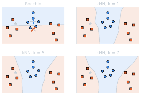
The choice of $k$ matters. With $k = 1$, the classifier copies the label of the single most similar document, which makes it sensitive to noise and to mislabeled training examples. Larger values smooth over noise, but if $k$ is too large, the neighborhood takes in documents from other classes and the classifier drifts toward predicting the most common classes. The example shows the second failure at small scale. Classifying each training point from the other thirteen, the leave-one-out test, kNN makes no errors with $k = 1$, 3, or 5, but 8 errors with $k = 7$, and all eight are B points. Each of B's clouds has only four points. Once one is held out, a B point's seven nearest neighbors are the three remaining points of its own cloud and then four A points, which are nearer than the far cloud, so A wins the vote. Rocchio, refitted without each held-out point, makes 9 leave-one-out errors. Small odd values such as 3 or 5 are common, and values from 10 to 100 are also used for text.
kNN's cost falls at classification time, when the new document must be compared with the training documents. With an inverted index over the training set, only training documents sharing a term with the new one are compared, using the same accumulation as computing vector scores. In effect, kNN classification is a search with the new document as the query.
A comparison on Reuters
The three classifiers were run on the ten largest Reuters-21578 categories, with the same training and test stories and the same text processing as in Naive Bayes classification. One binary classifier was built per category. For the vector space methods, documents were represented as length-normalized TF-IDF vectors with logarithmic term frequency. Rocchio compared a story's cosine similarity with two length-normalized centroids, one for the category's training stories and one for all other training stories. kNN weighted each neighbor's vote by its cosine similarity and assigned the category when the neighbors in it held more than half the total weight.
| Classifier | Micro-F1 | Macro-F1 |
|---|---|---|
| Rocchio | 0.715 | 0.593 |
| kNN, $k = 1$ | 0.745 | 0.703 |
| Multinomial Naive Bayes | 0.835 | 0.721 |
| kNN, $k = 5$ | 0.819 | 0.763 |
| kNN, $k = 10$ | 0.846 | 0.786 |
| kNN, $k = 30$ | 0.875 | 0.793 |
Rocchio did worst, as the diffuse "not in category" class predicts. With a single neighbor, kNN was noisy and fell below Naive Bayes on micro-F1. With 10 neighbors it edged past Naive Bayes on micro-F1 and clearly beat it on macro-F1, and with 30 it was the best of the three on both. Its macro-F1 of 0.793 at $k = 30$, against 0.721 for Naive Bayes, suggests that its advantage is larger on the small categories, which carry more weight in the macro average. A plausible reason is that kNN can follow the shape of a small class's region rather than averaging the class away.
How kNN depends on k
Sweeping $k$ from 1 to 100 shows the trade-off between noise and over-smoothing on real data (computed by tools/experiments/reuters/reuters_knn.py, which reproduces the table above):
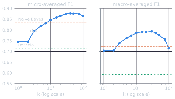
The two averages part company for large $k$. Micro-F1, dominated by the large categories, is almost flat from 30 to 100 neighbors, falling only to 0.864. Macro-F1 falls much faster, because the decision rule requires more than half of the neighbors' similarity weight to lie in the category. The smallest category, corn, has 181 training stories out of 7,769, and a corn story's 100 nearest neighbors increasingly include grain, wheat, and other stories that are not about corn. The neighborhood grows past the size of the class's region, which is the failure the example showed with $k = 7$. A per-category threshold, or $k$ chosen on held-out data, would soften it.
The per-category results show where the methods differ:
| Category | Rocchio F1 | kNN, $k = 30$, F1 |
|---|---|---|
| earn | 0.949 | 0.962 |
| acq | 0.907 | 0.863 |
| money-fx | 0.593 | 0.793 |
| grain | 0.599 | 0.818 |
| crude | 0.607 | 0.855 |
| trade | 0.319 | 0.751 |
| interest | 0.595 | 0.689 |
| ship | 0.578 | 0.713 |
| wheat | 0.433 | 0.788 |
| corn | 0.346 | 0.702 |
Rocchio is competitive only on the two largest categories, and on acq it beats kNN. Those categories hold nearly 60 percent of the training stories between them, so they are well described by their own centroid, and the "everything else" centroid of each is less diffuse than for a small category. On the small, overlapping categories, wheat, corn, and trade, Rocchio's F1 is about half of kNN's.
These results agree with the broader literature. In Yang and Liu's (1999) comparison on Reuters, support vector machines and kNN were the strongest of the methods tested, and Naive Bayes the weakest, with the largest differences on categories with few training examples. The comparison has limits. Naive Bayes was not tuned here, Rocchio's negative centroid could be improved, and kNN's threshold could be adjusted per category.
Linear classifiers and the bias-variance trade-off
Rocchio and Naive Bayes are both linear classifiers. Each defines, for a pair of classes, a hyperplane in the term space and assigns documents according to which side they fall on. They differ only in how they choose the hyperplane: Rocchio from the two centroids, as derived above, and Naive Bayes from the log ratios of term probabilities, as derived in Naive Bayes classification. Other linear methods choose it more directly. Support vector machines choose the hyperplane that separates the classes with the largest margin. Joachims (1998) found that they substantially outperformed the methods then standard for text, and they remained the strongest text classifiers for many years. Logistic regression chooses it to maximize the likelihood of the training labels and usually produces much better calibrated probabilities than Naive Bayes.
The comparison between linear classifiers and kNN illustrates the bias-variance trade-off (Manning, Raghavan, and Schütze, 2008, §14.6). A linear classifier has high bias: it can only draw a flat boundary, and it errs consistently where the true boundary is curved. In exchange it has low variance, since small changes in the training data move the boundary little. kNN has low bias, since it can follow any boundary, and high variance, since its decisions depend on exactly which training documents lie nearby.
Measured on simulated data
The trade-off can be measured where the true distribution is known. Two two-dimensional problems were simulated, each with class A a round Gaussian cloud centred at $(5, 6)$ with standard deviation 0.8:
- One cloud. Class B is a similar cloud centred at $(5, 4.2)$. The best possible boundary is the straight line $y = 5.1$, halfway between the centres, and even it misclassifies 13.0 percent of points, because the clouds overlap.
- Two clouds. Class B is split evenly between clouds at $(1.8, 5.2)$ and $(8.2, 5.2)$, like the example above. No straight line separates it from A.
For each problem, 30 training sets of 20 points per class were drawn with seeds 0 to 29, each classifier was trained on each, and its error was measured on the same 4,000 fresh points (2,000 per class). The table gives the median test error over the 30 runs, with the interquartile range:
| Classifier | One cloud, median (IQR) | Two clouds, median (IQR) |
|---|---|---|
| Rocchio | 0.129 (0.127–0.136) | 0.356 (0.335–0.373) |
| kNN, $k = 1$ | 0.188 (0.174–0.204) | 0.054 (0.047–0.069) |
| kNN, $k = 5$ | 0.146 (0.139–0.158) | 0.043 (0.039–0.048) |
| kNN, $k = 15$ | 0.135 (0.131–0.143) | 0.072 (0.060–0.110) |
On the one-cloud problem, where a straight line is the right shape, Rocchio is essentially optimal: its median error of 0.129 matches the best possible 0.130 (the difference is sampling noise in the test points), and its interquartile range is the narrowest in the table. kNN with one neighbor errs half again as often, because its boundary chases the particular training points it was given. On the two-clouds problem the roles reverse. Rocchio's bias dominates, and it misclassifies about a third of the points; since no straight line separates the classes, more data would not cure that. Meanwhile kNN with five neighbors errs on 4.3 percent. With 15 neighbors and only 20 points per class, about 10 in each of B's clouds, error rises again, plausibly for the reason the example showed: the neighborhoods are larger than a cloud and reach across into A.
The figure shows the variance directly, for the one-cloud problem:
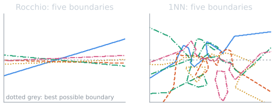
With a single neighbor, the variance dominates. Raising $k$ trades some of that variance for bias, and on Reuters the trade improved accuracy up to about $k = 30$. Which side of the trade-off wins depends on the data. Here, kNN's flexibility beat the two linear classifiers. But a well-trained linear classifier such as a support vector machine usually matches or beats kNN on text, whose many features make classes close to linearly separable, and it classifies far faster. Today, fine-tuned neural language models dominate it, by learning a nonlinear representation of the text on which a simple final layer can separate the classes.
References
- Joachims, T. (1998). Text categorization with support vector machines: Learning with many relevant features. In Proceedings of ECML 1998, 137–142.
- Manning, C. D., Raghavan, P., and Schütze, H. (2008). Introduction to Information Retrieval, chapter 14. Cambridge University Press.
- Yang, Y., and Liu, X. (1999). A re-examination of text categorization methods. In Proceedings of SIGIR 1999, 42–49.