A classifier that labels every Reuters story "not about corn" is right 98 percent of the time, since only 56 of the 3,019 test stories are about corn. It is also useless. Evaluating classifiers raises the problems familiar from retrieval evaluation, namely skewed classes and the inadequacy of accuracy, along with problems of its own. With many classes, results must be combined, and there are two ways to do it that answer different questions. A classifier's decisions depend on a threshold, and the threshold can matter as much as the classifier. And a classifier is built from data, so it must be evaluated on data it did not learn from. This article covers each, using the Reuters experiments from this topic. Unless stated otherwise, the classifier is multinomial Naive Bayes with add-one smoothing and all 18,135 terms, one binary classifier for each of the ten largest categories, and the numbers come from tools/experiments/reuters/reuters_more.py.
Per-class measures
For a binary classifier deciding whether documents belong to class $c$, each test document falls into one of four cells: true positive (TP), false positive (FP), false negative (FN), or true negative (TN), as in precision and recall. Precision is the fraction of documents assigned to $c$ that belong to it, $P = \mathrm{TP}/(\mathrm{TP} + \mathrm{FP})$. Recall is the fraction of documents in $c$ that were assigned to it, $R = \mathrm{TP}/(\mathrm{TP} + \mathrm{FN})$. F1 is their harmonic mean, $2PR/(P + R)$, which can also be written $2\,\mathrm{TP}/(2\,\mathrm{TP} + \mathrm{FP} + \mathrm{FN})$. True negatives appear in none of the three.
That omission is deliberate. For skewed classes true negatives dominate, so accuracy, $(\mathrm{TP} + \mathrm{TN})/N$, rewards doing nothing. The Naive Bayes classifier for corn has 48 true positives, 90 false positives, and 8 false negatives on the 3,019 test stories, which leaves 2,873 true negatives. Its accuracy is 0.968, below the 0.981 of the classifier that never says "corn", which looks better by accuracy but has F1 of zero. The corn classifier's F1 is 0.495, which says what the accuracy hides: it is wrong more often than right when it says "corn". Across the ten categories, accuracy ranges only from 0.939 to 0.985, while F1 ranges from 0.495 to 0.953.
Combining classes: micro and macro
A collection with many classes produces a precision, recall, and F1 for each. There are two ways to summarize them (Manning, Raghavan, and Schütze, 2008, §13.6; Sebastiani, 2002):
- Macro-averaging computes the measure for each class, then averages the per-class values. Every class counts equally.
- Micro-averaging pools the counts of all classes, the total true positives, false positives, and false negatives, into one table, then computes the measure once. Every positive decision and every missed positive counts equally, so large classes dominate.
The textbook's example has two classes:
| Class | True positives | False positives | Precision |
|---|---|---|---|
| Class 1 | 10 | 10 | 10/20 = 0.50 |
| Class 2 | 90 | 10 | 90/100 = 0.90 |
| Macro-averaged precision | (0.50 + 0.90)/2 = 0.70 | ||
| Micro-averaged precision | 100 | 20 | 100/120 = 0.83 |
The micro average is close to the large class's precision, and the macro average gives the small class equal weight.
Worked on Reuters
The full counts for the ten Reuters categories, sorted by size:
| Category | In test set | TP | FP | FN | Precision | Recall | F1 |
|---|---|---|---|---|---|---|---|
| earn | 1,087 | 1,051 | 79 | 36 | 0.930 | 0.967 | 0.948 |
| acq | 719 | 700 | 50 | 19 | 0.933 | 0.974 | 0.953 |
| crude | 189 | 180 | 71 | 9 | 0.717 | 0.952 | 0.818 |
| money-fx | 179 | 176 | 146 | 3 | 0.547 | 0.983 | 0.703 |
| grain | 149 | 142 | 109 | 7 | 0.566 | 0.953 | 0.710 |
| interest | 131 | 120 | 89 | 11 | 0.574 | 0.916 | 0.706 |
| trade | 117 | 104 | 170 | 13 | 0.380 | 0.889 | 0.532 |
| ship | 89 | 75 | 32 | 14 | 0.701 | 0.843 | 0.765 |
| wheat | 71 | 65 | 87 | 6 | 0.428 | 0.915 | 0.583 |
| corn | 56 | 48 | 90 | 8 | 0.348 | 0.857 | 0.495 |
| Pooled | 2,787 | 2,661 | 923 | 126 |
Micro-averaging pools the counts in the last row: precision $2{,}661/(2{,}661 + 923) = 0.742$, recall $2{,}661/(2{,}661 + 126) = 0.955$, and F1 $2 \times 2{,}661/(2 \times 2{,}661 + 923 + 126) = 0.835$.
Macro-averaging averages the columns: mean precision 0.612, mean recall 0.925, and mean F1 $(0.948 + 0.953 + \dots + 0.495)/10 = 0.721$.
The two F1 values, 0.835 and 0.721, differ by more than 0.1 for the same classifier on the same data. The two largest categories, earn and acq, together hold 65 percent of the positive test instances, 1,806 of 2,787, and are classified almost perfectly, so they dominate the pooled counts. Small categories such as corn and wheat score below 0.6, and in the macro average each counts as much as earn. The micro average says the classifier makes mostly correct decisions. The macro average says it is much weaker on small categories. Which matters depends on the application: a system routing news to desks of equal importance should care about the macro average, while one measuring the overall error rate of an automated pipeline might report the micro average. Reporting both is standard.
Macro-averaged F1 has two definitions in use. The one above averages the per-class F1 values. The other computes F1 from macro-averaged precision and recall, here $2 \times 0.612 \times 0.925/(0.612 + 0.925) = 0.737$. The two differ whenever classes differ in their balance of precision and recall, so a reported macro-F1 should say which it is. This topic uses the average of per-class F1 throughout.
The table also shows a pattern that the averages hide. Recall is above 0.84 for every category, while precision is below 0.6 for five of them. The classifier is not uniformly mediocre. It is systematically too willing to say yes, which is a problem of where its threshold sits, the subject of the next section.
The threshold and the precision-recall trade-off
A binary classifier usually computes a score and compares it with a threshold. Naive Bayes computes the log odds $\log \hat{P}(c \mid d)/\hat{P}(\bar{c} \mid d)$ and says yes when it is above 0, which corresponds to a posterior probability above 0.5. Nothing requires that threshold. Raising it makes the classifier say yes less often, which usually raises precision and lowers recall, and lowering it does the opposite. Sweeping the threshold over every score traces the classifier's whole range of behaviour, as a ranked list does in retrieval:
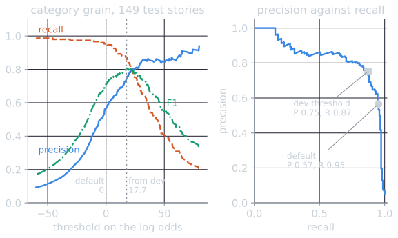
At the default threshold the grain classifier has precision 0.566, recall 0.953, and F1 0.710. The F1 curve peaks far to the right of zero. The threshold was therefore chosen properly, without looking at the test set: a classifier trained on 80 percent of the training stories (a random split, seed 790) scored the remaining 20 percent, and the threshold with the best F1 on them, a log odds of 17.7, was then applied to the classifier trained on all the training stories. On the test stories it gives precision 0.751, recall 0.872, and F1 0.807, an improvement of almost 0.1 from changing one number. The best threshold in hindsight, read off the test set, gives 0.808, so the development split found nearly all of what was available. The same procedure helped the other weak categories:
| Category | F1 at threshold 0 | Threshold from development split | F1 at that threshold |
|---|---|---|---|
| grain | 0.710 | 17.7 | 0.807 |
| wheat | 0.583 | 7.1 | 0.659 |
| corn | 0.495 | 8.4 | 0.570 |
| trade | 0.532 | 27.9 | 0.594 |
The best thresholds are log odds of 7 to 28, posterior probabilities from 0.999 to above $1 - 10^{-12}$, nowhere near the nominal 0.5. That is the poor calibration of Naive Bayes described in the Bernoulli model and why Naive Bayes works: its scores rank stories well, but their scale is wrong. Tuning the threshold on held-out data is the cheapest correction, and it is standard practice for text classifiers that make binary decisions. When a single number is wanted that does not depend on any threshold, the area under the precision-recall curve, or average precision over the ranking of test stories, summarizes the whole curve. For grain it is 0.833.
Multiclass problems
When each document belongs to exactly one of several classes, as with the star rating of a review, accuracy, the fraction of documents assigned the correct class, becomes meaningful again, because every document has one correct label. It is still incomplete. A confusion matrix, with true classes as rows and predicted classes as columns, shows which classes are confused with which. Per-class precision and recall, macro-averaged, show whether rare classes are handled at all.
Reuters can be turned into a multiclass problem by keeping only the stories that carry exactly one category label, from eight of the ten largest categories. (Wheat and corn drop out, since almost all their stories are also labeled grain.) That leaves 5,501 training and 2,190 test stories, and a single multinomial Naive Bayes classifier chooses one of the eight classes for each:
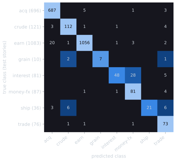
Accuracy is 0.952, against 0.495 for always predicting earn, the most common class. Macro-F1 is 0.852, and the matrix shows where the shortfall comes from. Only 48 of 81 interest stories are recognized, recall 0.593, and 28 of the rest are predicted as money-fx. Interest-rate stories and currency-market stories share much of their vocabulary, such as central banks, rates, and markets, and the classifier resolves the ambiguous ones toward money-fx. Ship has recall 0.583, with 6 stories predicted as crude, plausibly tanker traffic, and 6 as trade. Grain has only 10 single-label test stories, so its F1 of 0.824 rests on 3 errors. A single accuracy figure would show none of this.
For ordered classes, such as ratings from one to five stars, the confusion matrix reveals something accuracy hides. Predicting four stars for a five-star review is a smaller error than predicting one star, but accuracy counts both as simply wrong. Measures that account for distance, such as mean absolute error or weighted kappa, suit such problems better. The Goodreads project is an example.
Baselines
A score means little without a point of comparison. Useful baselines include:
- The majority class, always predicting the most common class. For skewed multiclass problems this can be strong. In the Goodreads project, 36.1 percent of reviews have four stars, so always predicting four stars is 36.1 percent accurate. On the single-label Reuters problem above it is 49.5 percent.
- Chance, predicting classes at random. For five equally likely classes, chance accuracy is 20 percent. This is the right comparison only when the classes are roughly balanced. When they are not, the majority-class baseline is the honest one.
- A simple standard method, such as Naive Bayes, which any more elaborate method should be shown to beat.
- A hand-written rule, where one is easy to write. For grain, the rule "the story contains grain, wheat, or corn" has F1 0.844 on the test stories, better than Naive Bayes at its default threshold (see the text classification problem).
A classifier's accuracy should be reported alongside the majority-class baseline, so that readers can see how much the classifier actually learned.
Train, test, and the cost of evaluating on training data
A classifier is fitted to its training data, so its performance on that data overstates its performance on new documents, a gap caused by overfitting. Reported results must come from a test set kept entirely apart from training, including from any tuning of parameters or selection of features (Manning, Raghavan, and Schütze, 2008, §13.6; Sebastiani, 2002).
The size of the gap can be measured directly. The Naive Bayes classifiers trained on Reuters were evaluated twice, once on the 7,769 training stories they were built from and once on the 3,019 held-out test stories:
| Evaluated on | Micro-F1 | Macro-F1 |
|---|---|---|
| The training stories | 0.861 | 0.772 |
| The held-out test stories | 0.835 | 0.721 |
Evaluating on training data overstated micro-F1 by 0.026 and macro-F1 by 0.051. The larger gap in the macro average suggests the inflation is greater for the small categories, where the classifier fits its few training examples most closely. Naive Bayes is a simple model, so its gap is modest. For flexible models, which can memorize their training data, evaluation on training data can be arbitrarily misleading. A 1-nearest-neighbor classifier evaluated on its own training documents finds each document as its own nearest neighbor and scores almost perfectly, whatever its accuracy on new documents.
Cross-validation
When labeled data is scarce, k-fold cross-validation makes better use of it. Divide the data into $k$ parts, train on $k - 1$ of them and test on the remaining one, rotate through all $k$ parts, and average the results (Sebastiani, 2002). Every document is used for testing exactly once, and never by a model that was trained on it. Any step that uses the labels must happen inside each training fold, as feature selection explains.
Cross-validation also shows how much a score depends on which documents happened to be tested. Ten-fold cross-validation on the 7,769 Reuters training stories (folds assigned at random, seed 742) gave these results for the ten folds:
| Measure | Mean over 10 folds | Lowest fold | Highest fold | Official test set |
|---|---|---|---|---|
| Micro-F1 | 0.822 | 0.812 | 0.836 | 0.835 |
| Macro-F1 | 0.719 | 0.684 | 0.743 | 0.721 |
The fold-to-fold spread is 0.024 in micro-F1 and 0.059 in macro-F1. Each fold holds about 777 stories, so a small category such as corn has only about 18 positive examples in a fold, and a few decisions move its F1, and with it the macro average, a long way. The official test set's scores fall inside the range of the folds. Differences between two classifiers smaller than this spread, measured on a single test set of similar size, should not be taken as evidence that one is better without a significance test.
For parameter tuning, a third set, a development set, is held out from training and used to choose parameters, so that the test set is touched only once, at the end. The threshold experiment above and the choice of the smoothing constant in Naive Bayes classification both work this way.
Beyond accuracy
As with retrieval, the measures here are proxies for what users need. A spam filter's costs are asymmetric, since losing a real message is worse than letting one spam message through, so its threshold should reflect the costs, as in the cost-sensitive Probability Ranking Principle. A classifier that routes documents to people for review should be judged by the reviewers' workload and what they miss, not by F1 alone. The measures in this article are the starting point for such judgments, not a substitute for them.
References
- Manning, C. D., Raghavan, P., and Schütze, H. (2008). Introduction to Information Retrieval, sections 13.6 and 14.5. Cambridge University Press.
- Sebastiani, F. (2002). Machine learning in automated text categorization. ACM Computing Surveys, 34(1), 1–47.