One percent of the documents in a collection are relevant to a query. A particular term appears in 80 percent of the relevant documents but only 5 percent of the others. If a document contains the term, how likely is it to be relevant? The answer, about 14 percent, follows from a few rules of probability. The same rules, applied term by term, produce the Binary Independence Model and the weight of every term in BM25. This article reviews the probability that the derivations in this topic rely on, using retrieval examples throughout and following Manning, Raghavan, and Schütze (2008, §11.1 and §11.3.2). The numbers in it are computed by tools/experiments/cranfield/probability_primer.py and rounded as shown.
Events, random variables, and the basic rules
A probability $P(A)$ measures how likely an event $A$ is, on a scale from 0 (impossible) to 1 (certain). Two rules follow from the axioms:
- The probabilities of all possible outcomes sum to 1.
- The complement of $A$, the event that $A$ does not happen, has probability $P(\bar{A}) = 1 - P(A)$.
A random variable assigns a value to each outcome. Many retrieval models use binary random variables. $R$ is 1 if a document is relevant and 0 if not, and $x_t$ is 1 if a document contains term $t$ and 0 if not. Writing $P(R = 1)$ means the probability that a document drawn at random is relevant.
Joint and conditional probability
The joint probability $P(A, B)$ is the probability that both $A$ and $B$ occur. The conditional probability $P(A \mid B)$ is the probability of $A$ given that $B$ is known to have occurred:
$$P(A \mid B) = \frac{P(A, B)}{P(B)}, \qquad \text{provided } P(B) > 0.$$
Conditioning restricts attention to the outcomes in which $B$ happened. $P(x_t = 1 \mid R = 1)$ is the fraction of relevant documents that contain $t$. $P(R = 1 \mid x_t = 1)$ is the fraction of documents containing $t$ that are relevant. These are different quantities, and confusing them is a common error in probabilistic reasoning. Retrieval needs the second, but data about relevant documents naturally gives the first.
Rearranging the definition gives the chain rule, $P(A, B) = P(A \mid B)\, P(B) = P(B \mid A)\, P(A)$. It extends to any number of events:
$$P(A, B, C) = P(A \mid B, C)\, P(B \mid C)\, P(C).$$
The law of total probability splits an event by cases: $P(B) = P(B \mid A)\, P(A) + P(B \mid \bar{A})\, P(\bar{A})$.
Bayes' rule
Equating the two forms of the chain rule and dividing by $P(B)$ gives Bayes' rule, which turns one conditional probability into the other:
$$P(A \mid B) = \frac{P(B \mid A)\, P(A)}{P(B)}.$$
$P(A)$ is the prior probability of $A$, before $B$ is observed. $P(A \mid B)$ is the posterior, after. $P(B \mid A)$ is the likelihood of the evidence under $A$.
For the opening example, the prior probability of relevance is $P(R = 1) = 0.01$, the term appears in relevant documents with probability $P(x_t = 1 \mid R = 1) = 0.8$, and in nonrelevant documents with probability $P(x_t = 1 \mid R = 0) = 0.05$. By Bayes' rule, with the denominator expanded by total probability,
$$P(R = 1 \mid x_t = 1) = \frac{0.8 \times 0.01}{0.8 \times 0.01 + 0.05 \times 0.99} = \frac{0.008}{0.0575} \approx 0.139.$$
The term is strong evidence, since it is sixteen times as common in relevant documents, yet a document containing it is still more likely nonrelevant than relevant. The prior is so low that even strong evidence leaves the posterior at 14 percent. That is typical of retrieval: relevant documents are rare, so any single clue is weak, and models must combine many clues.
The same calculation as counts
Bayes' rule is easier to trust when it is done with counts. Imagine 10,000 documents with exactly the stated proportions:
| Contain the term | Lack the term | Total | |
|---|---|---|---|
| Relevant | 80 | 20 | 100 |
| Nonrelevant | 495 | 9,405 | 9,900 |
| Total | 575 | 9,425 | 10,000 |
Each row applies one conditional probability: 80 percent of the 100 relevant documents contain the term, and 5 percent of the 9,900 nonrelevant ones do. The question "how likely is a document containing the term to be relevant?" reads down the first column: 80 of the 575 documents that contain the term are relevant, and $80 / 575 = 0.139$. The 495 nonrelevant documents outnumber the 80 relevant ones because there are 99 times as many nonrelevant documents to begin with. Bayes' rule is exactly this division, written with probabilities instead of counts. The same table answers the opposite question as well: a document that lacks the term is relevant with probability $20 / 9425 = 0.0021$, a fifth of the prior. The absence of a good term is evidence too, and the BIM uses it.
How the prior controls the answer
The posterior depends as much on the prior as on the evidence. The figure plots the posterior against the prior for three strengths of evidence: the term above, a second term discussed below, and both together.
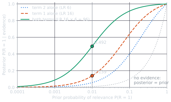
For a fixed query the prior is the same for every document, so it does not change the order in which documents are ranked. It does decide whether a score can be read as a probability. That distinction between ranking and calibration returns in the Probability Ranking Principle.
Odds and log odds
The odds of an event are the ratio of its probability to the probability of its complement:
$$O(A) = \frac{P(A)}{1 - P(A)}.$$
A probability of 0.5 is odds of 1. Odds range from 0 to infinity, and they increase whenever the probability does, so ranking by odds gives the same order as ranking by probability. In odds form, Bayes' rule becomes a multiplication. Writing Bayes' rule once for $R = 1$ and once for $R = 0$ and dividing the two, the denominator $P(x_t)$ cancels:
$$O(R \mid x_t) = \frac{P(R = 1 \mid x_t)}{P(R = 0 \mid x_t)} = \frac{P(x_t \mid R = 1)\, P(R = 1) / P(x_t)}{P(x_t \mid R = 0)\, P(R = 0) / P(x_t)} = O(R) \times \frac{P(x_t \mid R = 1)}{P(x_t \mid R = 0)}.$$
The second factor is the likelihood ratio. In the example, the prior odds are $0.01/0.99 \approx 0.0101$, the likelihood ratio is $0.8/0.05 = 16$, and the posterior odds are $0.0101 \times 16 \approx 0.162$, which corresponds to the probability 0.139 found above (converting back, $p = O / (1 + O)$). In the table of counts, the posterior odds are simply $80 : 495$. The troublesome denominator $P(x_t)$ has disappeared, which is exactly why the BIM derivation ranks by odds rather than probability.
Taking logarithms turns the multiplication into addition:
$$\log O(R \mid x_t) = \log O(R) + \log \frac{P(x_t \mid R = 1)}{P(x_t \mid R = 0)}.$$
Evidence now adds. Each piece of evidence contributes its log likelihood ratio, and a ranking function becomes a sum of term weights. The logarithm also preserves order, so the ranking is still unchanged.
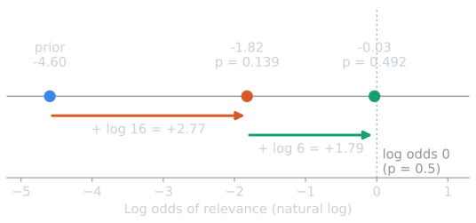
On this scale a term weight is a distance, and a document's score is where its evidence carries it. A term that is equally common in relevant and nonrelevant documents has likelihood ratio 1 and weight 0. A term that is rarer in relevant documents has a negative weight and moves the score left.
Conditional independence
Two events are independent if $P(A, B) = P(A)\, P(B)$. They are conditionally independent given $C$ if
$$P(A, B \mid C) = P(A \mid C)\, P(B \mid C).$$
The BIM and Naive Bayes assume that terms are conditionally independent given relevance. Then the likelihood ratio for a whole document is the product of the per-term ratios, and the log odds are a sum of per-term weights.
Suppose a second term appears in 60 percent of relevant documents and 10 percent of nonrelevant ones, a likelihood ratio of 6. If the two terms are conditionally independent given relevance, a document containing both has posterior log odds
$$\log 0.0101 + \log 16 + \log 6 = -4.5951 + 2.7726 + 1.7918 \approx -0.031,$$
using natural logarithms. That corresponds to odds of 0.970 and a probability of 0.492. Two pieces of evidence that are each strong but individually insufficient together raise a 1 percent prior to nearly even odds. Real terms are not conditionally independent, since terms about the same subject tend to occur together, so this calculation overcounts correlated evidence. The models work anyway because ranking depends only on the order of the scores, a point taken up in the BIM article.
Two kinds of independence
Conditional independence and plain independence are different claims, and neither implies the other. In the example, the two terms are independent within the relevant documents and within the nonrelevant documents, by assumption. Across the whole collection they are not:
$$P(t_1, t_2) = 0.01 \times 0.8 \times 0.6 + 0.99 \times 0.05 \times 0.1 = 0.00975,$$
while $P(t_1)\, P(t_2) = 0.0575 \times 0.105 = 0.00604$. The terms co-occur 1.61 times as often as independence predicts, purely because both are more common in the relevant documents. Relevance is a common cause, and conditioning on it removes the association it creates. That is what the BIM assumes: whatever links terms together runs through relevance.
Testing the assumption on real counts
The Cranfield collection of 1,400 aerodynamics abstracts (the collection used throughout this topic, analyzed as in comparing ranking models) shows how far real terms are from this ideal. Panel occurs in 45 abstracts and flutter in 56. If they occurred independently, about $45 \times 56 / 1400 = 1.8$ abstracts would contain both. In fact 20 do, eleven times as many: panel flutter is a named phenomenon. Conditioning on relevance does not remove the association either. Among the 1,391 abstracts not relevant to Cranfield query 185, experimental studies on panel flutter, 11 contain both words where independence within that class predicts 1.2. The terms are associated because they name one subject, and that subject is shared by relevant and nonrelevant documents alike.
The consequence for a model that assumes conditional independence is double counting. A document containing both words receives credit for panel and again for flutter, although the second word adds less information than its weight claims, because it nearly always accompanies the first. For ranking, the damage is limited when the overcounting is similar across the documents being compared. All the abstracts that mention panel flutter are inflated together. How the BIM fares on this very query is worked through in the BIM article.
Estimating probabilities from counts
Models need numbers for quantities like $P(x_t = 1 \mid R = 1)$. The natural estimate is a relative frequency. If 8 of 10 known relevant documents contain $t$, estimate 0.8. This is the maximum likelihood estimate, the value that makes the observed data most probable.
Maximum likelihood estimates fail on small samples. If none of 10 relevant documents contains a term, the estimate is 0, and a log odds weight becomes infinite. If all 10 contain it, $1 - p = 0$ and the weight is again infinite. Smoothing adds a small pseudo-count to each outcome so that no estimate is exactly 0 or 1. Adding $\tfrac{1}{2}$ to each count, as in the Robertson–Spärck Jones weight (Robertson and Spärck Jones, 1976), gives
$$\hat{p} = \frac{s + \tfrac{1}{2}}{S + 1}$$
for a term in $s$ of $S$ relevant documents. Adding 1 instead (Laplace smoothing) is common in Naive Bayes. Both can be justified as Bayesian estimates under a prior belief about the probability, and both pull small-sample estimates toward the middle, which is what a careful estimate from little evidence should do.
With only four judged relevant documents, the three estimators disagree sharply at the extremes:
| Relevant documents containing $t$ ($s$ of 4) | 0 | 1 | 2 | 3 | 4 |
|---|---|---|---|---|---|
| Maximum likelihood $s/S$ | 0.000 | 0.250 | 0.500 | 0.750 | 1.000 |
| Add $\tfrac12$: $(s + \tfrac12)/(S + 1)$ | 0.100 | 0.300 | 0.500 | 0.700 | 0.900 |
| Add 1: $(s + 1)/(S + 2)$ | 0.167 | 0.333 | 0.500 | 0.667 | 0.833 |
| Log odds $\log \frac{p}{1-p}$, add $\tfrac12$ | −2.197 | −0.847 | 0.000 | 0.847 | 2.197 |
Under maximum likelihood the outer columns give log odds of minus and plus infinity, so one term absent from four documents would veto a document outright. The smoothed estimates keep the weight finite and say, in effect, that four observations are not enough to be certain.
Where the pseudo-counts come from
The Bayesian justification can be derived in a few lines. Treat the unknown probability $p$ as a random variable with a Beta prior, whose density is proportional to $p^{\alpha - 1} (1 - p)^{\alpha - 1}$. With $\alpha = 1$ this is uniform: every value of $p$ equally plausible.
- Likelihood. Observing the term in $s$ of $S$ documents has probability proportional to $p^{s} (1 - p)^{S - s}$.
- Posterior. By Bayes' rule the posterior density is proportional to prior times likelihood, $p^{s + \alpha - 1} (1 - p)^{S - s + \alpha - 1}$. This is again a Beta density, with the counts added to the prior's parameters. That is why the prior's parameter behaves like a count.
- Posterior mean. The mean of a Beta density proportional to $p^{a - 1}(1 - p)^{b - 1}$ is $a / (a + b)$. Here that gives
$$E[p \mid s, S] = \frac{s + \alpha}{S + 2\alpha}.$$
With $\alpha = 1$ this is add-one (Laplace) smoothing, and with $\alpha = \tfrac12$ it is the add-a-half estimate above. Numerically integrating the posterior for $s = 1$ of $S = 4$ reproduces 0.300 and 0.333. A larger $\alpha$ expresses a stronger prior belief that $p$ is near one half, and needs more data to overcome. Manning, Raghavan, and Schütze (2008, §11.3.2 and §11.3.4) present the same idea and use it again in relevance feedback, where the previous estimate of $p_t$ serves as the prior for the next.
The quantities this topic uses
| Quantity | Meaning |
|---|---|
| $P(R = 1 \mid d, q)$ | What the Probability Ranking Principle says to rank by |
| $O(R \mid d, q)$ | The same ranking, without the hard-to-estimate denominator |
| $p_t = P(x_t = 1 \mid R = 1)$ | How often relevant documents contain term $t$ |
| $u_t = P(x_t = 1 \mid R = 0)$ | How often nonrelevant documents contain $t$, close to $\mathit{df}_t / N$ |
| $\log \frac{p_t (1 - u_t)}{u_t (1 - p_t)}$ | The log odds ratio weight of term $t$ in the BIM |
References
- Manning, C. D., Raghavan, P., and Schütze, H. (2008). Introduction to Information Retrieval, sections 11.1 and 11.3. Cambridge University Press.
- Robertson, S. E., and Spärck Jones, K. (1976). Relevance weighting of search terms. Journal of the American Society for Information Science, 27(3), 129–146.