Cut two permutations of the cities 1 to 9 at the same point and swap their tails, as one-point crossover does with bit strings:
parents   1 2 3 | 4 5 6 7 8 9      9 3 7 | 8 2 6 5 1 4
child     1 2 3 | 8 2 6 5 1 4
The child visits cities 1 and 2 twice and never visits 7 or 9. It is not a tour at all. A variation operator is only meaningful for a particular representation: it must turn valid genotypes into valid genotypes, and it should turn good ones into ones that are likely to be good. This article describes the standard crossover (recombination) and mutation operators for the three representations a genetic algorithm most often uses, bit strings, real-valued vectors and permutations, following the organization of Eiben and Smith (2015, ch. 4). Every worked example is printed by the script tools/experiments/evolution/operators.py in the site repository, and the figures, with the numbers computed from them, by tools/figures/crossover-and-mutation-operators.py. How strongly the population is pushed toward its best members, the other half of the search, is the subject of selection pressure and premature convergence.
Binary strings
One-point, two-point and uniform crossover
Take two parents of length 8, with positions numbered 1 to 8 from the left:
A = 11010011 B = 01101100
One-point crossover chooses a cut point and swaps everything after it. Cutting after position 3 gives the children 11001100 and 01110011. Two-point crossover chooses two cut points and swaps the segment between them; cutting after positions 2 and 6 swaps positions 3 to 6 and gives 11101111 and 01010000. $n$-point crossover generalizes this to $n$ cuts, swapping alternate segments.
Uniform crossover decides every position independently. A random mask says, for each position, which parent the first child takes its bit from; the second child takes the other. With the mask 10110010, where 1 means "from A", the children are 11011110 and 01100001. Syswerda (1989) presented uniform crossover and compared it, theoretically and empirically, with one-point and two-point crossover. Each mask bit is usually 1 with probability 0.5.
The figure draws the three examples cell by cell. In every case the two children between them hold exactly the bits of the two parents at each position, one from each; the operators differ only in the pattern that decides which child gets which.
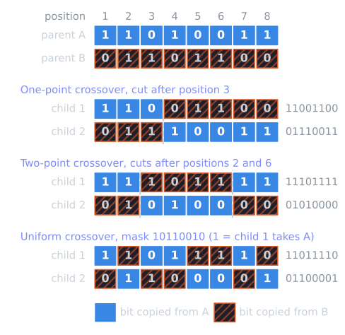
All three operators only rearrange existing values. At a position where both parents carry the same bit, every child carries it too. Crossover can therefore never restore a value that has disappeared from the population; that is mutation's job.
Positional bias and disruption
The operators differ in which genes they keep together. Under one-point crossover, two positions are separated only if the cut falls between them, so adjacent positions almost always travel together and the two ends of the string are always separated. Under uniform crossover, distance along the string makes no difference. Eshelman, Caruana and Schaffer (1989) called this dependence on distance positional bias, and distinguished it from distributional bias, a bias in how many positions are exchanged: one-point crossover exchanges any number from 1 to $L - 1$ with equal probability, while uniform crossover exchanges a binomially distributed number, concentrated around $L/2$.
Positional bias decides how often crossover breaks up a combination of values that makes an individual good. In the terms of Holland's schema theorem, a schema is a pattern of fixed values at certain positions, and crossover disrupts it when neither child inherits all of those values from the same parent. The script computes the probability exactly, by enumerating every cut point or mask, for strings of length $L = 10$, assuming the other parent differs from the first at every fixed position (the worst case):
| Fixed positions | One-point | Two-point | Uniform |
|---|---|---|---|
| 1, 2 | 0.111 | 0.222 | 0.500 |
| 1, 5 | 0.444 | 0.556 | 0.500 |
| 4, 7 | 0.333 | 0.500 | 0.500 |
| 1, 10 | 1.000 | 0.000 | 0.500 |
| 1, 5, 10 | 1.000 | 0.556 | 0.750 |
Each column of the table follows from counting, and the counts are worth doing once, because they explain the shapes.
One-point. There are $L - 1$ places to cut, after position 1 through after position $L - 1$, each chosen with probability $1/(L - 1)$. Two fixed positions $i < j$ end up in different children exactly when the cut falls after one of the positions $i, i + 1, \dots, j - 1$, which are $j - i$ of the $L - 1$ places. The defining length $\delta$ of a schema is the distance between its outermost fixed positions, $j - i$, so the probability of disruption is
$$P_{\text{one}} = \frac{\delta}{L - 1}.$$
Fixed positions in between do not matter: if the outermost two stay together, so does everything between them. One cut in nine falls between positions 1 and 2, giving 0.111, and every cut falls between 1 and 10, giving 1.
Two-point. Now two distinct cut places are drawn from the same $L - 1$, giving $\binom{L - 1}{2}$ equally likely pairs, and the segment between them is swapped. Positions $i$ and $j$ are separated when exactly one of the two cuts falls among the $\delta$ places between them: if neither does, both positions are on the same side of the segment; if both do, the segment lies strictly between them and both again stay with the same parent. Choosing one cut among the $\delta$ inner places and the other among the $L - 1 - \delta$ outer ones gives
$$P_{\text{two}} = \frac{\delta \, (L - 1 - \delta)}{\binom{L - 1}{2}}.$$
For $L = 10$ the denominator is 36. Positions 1 and 2 ($\delta = 1$) are separated with probability $1 \cdot 8/36 = 0.222$, twice the one-point value, while positions 1 and 10 ($\delta = 9$) give $9 \cdot 0 / 36 = 0$. Two-point crossover behaves as if the string were a ring: positions 1 and 10 are never separated, because any segment between two cuts leaves both ends on the same side. On a ring, positions 1 and 10 are neighbours, and the formula is symmetric under $\delta \to L - 1 - \delta$. The figure script checks the formula against enumeration for every $\delta$ from 1 to 9.
Uniform. Each position independently goes to child 1 from parent A with probability 1/2. A schema with $k$ fixed positions survives in child 1 if all $k$ come from A, or all from B, which has probability $2 \cdot 2^{-k} = 2^{-(k-1)}$. The disruption probability is $1 - 2^{-(k-1)}$, independent of where the positions are: 0.5 for $k = 2$ and 0.75 for $k = 3$.
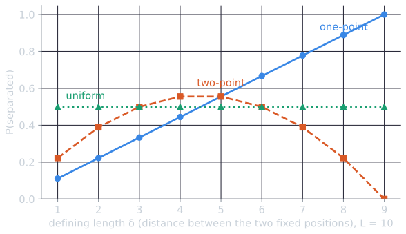
None of the operators is better in general. Low disruption helps when good combinations are encoded close together, as the building block hypothesis assumes; high disruption helps the search explore, and treats all positions alike when the encoding gives no reason to prefer an order. Which matters more depends on the encoding and the problem.
Bit-flip mutation
Bit-flip mutation flips each bit independently with probability $p_m$. The common default $p_m = 1/L$ flips one bit on average. It is also the rate used in the standard analysis of the (1+1) EA, which keeps one parent and accepts its mutant if it is no worse; with $p_m = 1/L$, its expected time to optimize any linear function of $L$ bits is $\Theta(L \log L)$ (Droste, Jansen and Wegener, 2002). Flipping positions 2 and 7 of 11001100 gives 10001110.
At $p_m = 1/L$ a sizable fraction of offspring are not mutated at all. The probability of no flip is $(1 - 1/L)^L$, which approaches $1/e$:
| $L$ | P(no flip) | P(exactly one flip) |
|---|---|---|
| 8 | 0.3436 | 0.3927 |
| 20 | 0.3585 | 0.3774 |
| 100 | 0.3660 | 0.3697 |
About a third of all offspring are copies of their crossover result, which matters when evaluations are expensive and when diversity is already low.
How the mutation rate shapes a run
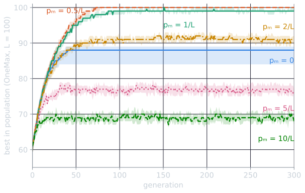
The rate $1/L$ is a default, not a law, and what happens on either side of it is easy to see on the simplest problem there is. OneMax asks for a string of $L$ bits with as many ones as possible, so the fitness of a string is its number of ones and the optimum is the all-ones string. The script tools/experiments/evolution/mutation_rate.py runs a generational GA on OneMax with $L = 100$: a population of 50, binary tournament selection, two-point crossover with probability 0.9, bit-flip mutation at rate $p_m$, and complete replacement of the population each generation with no elitism, so that even the best string can be lost. Each of six rates was run for 300 generations with the same 30 seeds.
| $p_m$ | Mutated bits per child | Best in final population, median [IQR] | Runs ever reaching 100 |
|---|---|---|---|
| 0 | 0 | 88 [84, 89] | 0 of 30 |
| $0.5/L$ | 0.5 | 100 [100, 100] | 30 of 30 |
| $1/L$ | 1 | 99 [99, 100] | 30 of 30 |
| $2/L$ | 2 | 91 [89.25, 92] | 0 of 30 |
| $5/L$ | 5 | 76.5 [76, 77] | 0 of 30 |
| $10/L$ | 10 | 68 [67, 70] | 0 of 30 |
The two ends of the table fail for opposite reasons.
Without mutation, the population runs out of material. Selection and crossover only reshuffle the bits the initial population contains, and in a finite population a position can lose its last 1 by chance, through a tournament that happens not to pick the strings carrying it. Once lost, it can never return. In the final populations of the $p_m = 0$ runs a median of 12 positions held no 1 anywhere, and the best string, at 88, is exactly $100 - 12$: every remaining position had been fixed at 1. De Jong saw a stall of the same kind, a population converged at most positions, in his own runs, described in the De Jong functions article.
With too much mutation, the population cannot hold what it finds. A child with $f$ ones has $L - f$ zeros, each turned into a one with probability $p_m$, and $f$ ones, each turned into a zero with the same probability. Its expected change from mutation alone is therefore
$$p_m (L - f) - p_m f = p_m (L - 2f),$$
which is negative whenever more than half of the bits are already right. At $p_m = 5/L = 0.05$ and $f = 76.5$, the median final value, a child loses $0.05 \times (100 - 153) = 2.65$ ones on average. The population levels off where the gain from selection each generation balances that loss, a mutation-selection balance, and the balance point falls as $p_m$ rises: the expected loss at the final median is 1.64 for $2/L$ and 3.60 for $10/L$. Even at $1/L$ the effect is visible. Every one of the 30 runs found the optimum, but a child of the all-ones string survives mutation unchanged only with probability $(1 - 1/L)^L = 0.366$, and with no elitism the final population still held it in only 10 of the 30 runs, hence the median of 99. Halving the rate to $0.5/L$ reached the optimum sooner (median generation 70 against 92.5) and kept it in all 30.
These numbers belong to this GA. OneMax rewards every single correct bit, so small steps are always enough, and keeping the best individual (elitism), which this GA deliberately does not do, would at least stop it from losing the best string it has found. On problems with local optima that only a multi-bit jump can leave, a higher rate can pay for itself, which is part of why no rate is best for all problems.
With the standard binary code, a single flip can change the decoded value by a large or a small amount depending on which bit flips, and adjacent values such as 7 (0111) and 8 (1000) differ in every bit. These Hamming cliffs, and the Gray code that removes them, are covered in binary encoding and Gray codes.
Real-valued vectors
When the variables are real numbers, a vector of floating-point values avoids the precision limit and the Hamming cliffs of a binary encoding. The operators below act on one variable at a time; for a vector they are applied to each variable, or to a randomly chosen subset. The worked examples use the parents $p_1 = 2$ and $p_2 = 5$.
Arithmetic and linear crossover
Arithmetic recombination takes a weighted average. In the whole-arithmetic form described by Eiben and Smith (2015, ch. 4), the children are $c_1 = \alpha p_1 + (1 - \alpha) p_2$ and $c_2 = (1 - \alpha) p_1 + \alpha p_2$; with $\alpha = 0.25$ they are 4.25 and 2.75. The children always lie between the parents, so repeated arithmetic crossover shrinks the population's spread, and the population cannot move outside the range it started in by crossover alone.
Linear crossover (Wright, 1991) generates three candidates, the midpoint and two points beyond the parents on the line through them:
$$\tfrac{1}{2} p_1 + \tfrac{1}{2} p_2, \qquad \tfrac{3}{2} p_1 - \tfrac{1}{2} p_2, \qquad -\tfrac{1}{2} p_1 + \tfrac{3}{2} p_2,$$
here 3.5, 0.5 and 6.5. The usual description keeps the best two of the three, which costs three evaluations per crossover.
Blend crossover (BLX-α)
Blend crossover (Eshelman and Schaffer, 1993) draws each child uniformly from an interval that extends beyond the parents on both sides by a fraction $\alpha$ of their distance. With $d = |p_2 - p_1|$, the interval is
$$\left[ \min(p_1, p_2) - \alpha d, \; \max(p_1, p_2) + \alpha d \right].$$
For $\alpha = 0.5$ and the parents 2 and 5 the interval is $[0.5, 6.5]$, and a uniform random number $u = 0.3$ gives the child $0.5 + 0.3 \times 6 = 2.3$. The endpoints at $\alpha = 0.5$ are exactly Wright's two outer points, $\tfrac{3}{2} p_1 - \tfrac{1}{2} p_2$ and its mirror. BLX-0.5 is a common setting; Deb and Agrawal (1995) used it as the real-coded baseline when they introduced simulated binary crossover.
Simulated binary crossover (SBX)
Simulated binary crossover (Deb and Agrawal, 1995) was designed to give a real-valued GA the search behaviour of one-point crossover on binary strings. Deb and Agrawal observed two properties of one-point crossover on decoded values. The mean of the two children equals the mean of the parents. And the spread factor
$$\beta = \frac{|c_2 - c_1|}{|p_2 - p_1|},$$
the ratio of the children's distance to the parents' distance, is usually close to 1: children near the parents are more likely than children far away. They modelled the distribution of $\beta$ with a polynomial,
$$\mathcal{P}(\beta) = \begin{cases} 0.5 (\eta + 1) \beta^{\eta}, & \beta \le 1, \\ 0.5 (\eta + 1) \dfrac{1}{\beta^{\eta + 2}}, & \beta > 1, \end{cases}$$
where the distribution index $\eta \ge 0$ controls the spread. Each branch carries probability 0.5, so contracting ($\beta < 1$) and expanding ($\beta > 1$) crossovers are equally likely. A large $\eta$ concentrates $\beta$ near 1, putting children close to their parents; a small $\eta$ spreads them out. Deb and Agrawal reported that values from 2 to 5 matched the behaviour of one-point crossover in their simulations.
To sample $\beta$, draw $u$ uniformly from $[0, 1)$ and invert the cumulative distribution $F(\beta) = \int_0^{\beta} \mathcal{P}(b) \, db$. On the contracting branch,
$$F(\beta) = \int_0^{\beta} 0.5 (\eta + 1) b^{\eta} \, db = 0.5\, \beta^{\eta + 1}, \qquad \beta \le 1,$$
which reaches 0.5 at $\beta = 1$. On the expanding branch the first half is already accumulated, and
$$F(\beta) = 0.5 + \int_1^{\beta} 0.5 (\eta + 1) b^{-(\eta + 2)} \, db = 0.5 + 0.5 \left( 1 - \beta^{-(\eta + 1)} \right) = 1 - 0.5\, \beta^{-(\eta + 1)}, \qquad \beta > 1.$$
Setting $F(\beta) = u$ and solving each branch for $\beta$ gives
$$\beta = \begin{cases} (2u)^{1/(\eta + 1)}, & u \le 0.5, \\ \left( \dfrac{1}{2(1 - u)} \right)^{1/(\eta + 1)}, & u > 0.5. \end{cases}$$
The children are then placed symmetrically about the parents' mean:
$$c_1 = \tfrac{1}{2} \left[ (1 + \beta) p_1 + (1 - \beta) p_2 \right], \qquad c_2 = \tfrac{1}{2} \left[ (1 - \beta) p_1 + (1 + \beta) p_2 \right].$$
With $\eta = 2$ and $u = 0.3$, $\beta = 0.6^{1/3} = 0.8434$, a contracting crossover, and the children are 2.2349 and 4.7651. With $u = 0.8$, $\beta = 2.5^{1/3} = 1.3572$, an expanding one, and the children are 1.4642 and 5.5358. In both cases the children sum to 7, as the parents do, and their distance is $\beta$ times the parents' distance of 3.
Deb and Agrawal found that real-coded GAs using SBX performed as well as or better than binary-coded GAs with one-point crossover on the test problems they studied. Because the children's spread is proportional to the parents' distance, SBX searches widely while the population is spread out and finely once it has converged. Deb and Beyer (2001) showed that this gives a real-valued GA with SBX, even without mutation, a self-adaptive behaviour similar to that of self-adaptive evolution strategies. BLX-α shares the property.
Implementations differ in a detail the formulas above leave open. For a vector of variables, the pair of values that SBX produces for each variable can be assigned to the two children in a fixed order, as written here, or swapped at random for each variable, as in Deb's own NSGA-II code. The swap mixes the two parents' variables between children much as uniform crossover does, and it can change results substantially: in the NSGA-II article's experiments, it changes the median generational distance on ZDT1 by more than two orders of magnitude.
Mutation for real values
Uniform mutation replaces a value with one drawn uniformly from the variable's range. Gaussian mutation adds normally distributed noise, $x' = x + \sigma z$ with $z$ drawn from the standard normal distribution; with $x = 3$, $\sigma = 0.5$ and $z = -1.2$, $x' = 2.4$. The step size $\sigma$ is the critical parameter, and evolution strategies adapt it during the run, as described in the 1/5 success rule.
Polynomial mutation (Deb and Goyal, 1996) applies the same idea as SBX to a single parent. With a variable bounded by $[x_L, x_U]$, a distribution index $\eta_m$, and $u$ drawn uniformly from $[0, 1)$, the basic form is
$$\delta = \begin{cases} (2u)^{1/(\eta_m + 1)} - 1, & u < 0.5, \\ 1 - \left[ 2(1 - u) \right]^{1/(\eta_m + 1)}, & u \ge 0.5, \end{cases} \qquad x' = x + \delta \, (x_U - x_L).$$
The perturbation $\delta$ lies in $[-1, 1)$ and is concentrated near 0, more strongly as $\eta_m$ grows. For $x = 3$ in $[0, 10]$:
| $\eta_m$ | $u$ | $\delta$ | $x'$ |
|---|---|---|---|
| 2 | 0.7 | +0.1566 | 4.5657 |
| 2 | 0.2 | −0.2632 | 0.3681 |
| 20 | 0.7 | +0.0240 | 3.2403 |
| 20 | 0.2 | −0.0427 | 2.5731 |
The basic form can push a value outside its bounds; implementations clip it, or use a later variant whose distribution depends on the distance to each bound.
Where the children land
Writing $m = (p_1 + p_2)/2$ for the parents' mean and $d = p_2 - p_1$ for their distance, the SBX formulas simplify to $c_1 = m - \beta d / 2$ and $c_2 = m + \beta d / 2$. A child at distance $\lvert c - m \rvert$ from the mean therefore corresponds to $\beta = 2 \lvert c - m \rvert / d$, and changing variables turns the density of $\beta$ into the density of a child, picked at random from the pair:
$$g(c) = \frac{1}{d} \, \mathcal{P}\!\left( \frac{2 \lvert c - m \rvert}{d} \right).$$
Where $\beta = 1$, at $c = p_1$ and $c = p_2$, the density peaks. BLX-α has a flat density instead, $1/((1 + 2\alpha) d)$ over its interval. The figure plots both for the parents 2 and 5, together with the density of polynomial mutation, which by the same change of variables is $(\eta_m + 1)(1 - \lvert \delta \rvert)^{\eta_m} / (2 (x_U - x_L))$ at $x' = x + \delta (x_U - x_L)$.
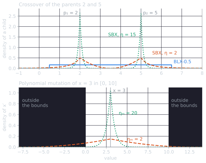
The shapes have practical consequences, which the figure script computes from the densities and checks against a million samples of each operator:
- Under BLX-0.5, half the children land outside the interval between the parents, a quarter on each side, and the children are spread evenly. Under SBX the share between the parents is also exactly one half, because contracting and expanding crossovers are equally likely, but the children concentrate near the parents. With $\eta = 2$, a child lands within 0.5 of the midpoint 3.5 with probability only 0.019, and within $[1, 6]$ with probability 0.892.
- SBX treats the two parents as two centres. When they are far apart, the children stay near one or the other; SBX does not average two solutions into a compromise between them, as arithmetic recombination does.
- Polynomial mutation of $x = 3$ in $[0, 10]$ with $\eta_m = 2$ sends a mutant outside the range with probability $0.5 (0.7)^3 + 0.5 (0.3)^3 = 0.185$, so the clipping mentioned above is not a corner case: clipped mutants pile up on the bound. With $\eta_m = 20$ the probability is 0.0003, and two-thirds of the mutants (0.659) move by less than 0.5.
Permutations
Many combinatorial problems, such as the travelling salesman problem and job scheduling, ask for an ordering. A permutation representation needs operators that always produce permutations, which the example at the start of this article shows one-point crossover does not. The examples below use the parents
P1 = 1 2 3 4 5 6 7 8 9 P2 = 9 3 7 8 2 6 5 1 4
and the segment from position 4 to position 7.
Partially mapped crossover (PMX)
Partially mapped crossover (Goldberg and Lingle, 1985) copies a segment from one parent and fills the rest from the other parent at the same positions, repairing duplicates through the correspondence that the segment defines. The child starts with P1's segment, 4 5 6 7, at positions 4 to 7. Every other position takes P2's value at that position unless that value is already in the segment:
- Positions 1, 2 and 8 take P2's values 9, 3 and 1, which are not in the segment.
- Position 3 would take 7, which is already present. In the segment, P1's 7 sits where P2 has 5, so 7 maps to 5; 5 is also in the segment and maps, in the same way, to 2. Position 3 takes 2.
- Position 9 would take 4, which maps to 8. Position 9 takes 8.
The child is 9 3 2 4 5 6 7 1 8. PMX is also often implemented as a sequence of swaps: start from a copy of P2 and, for each position in the segment, swap P1's value into that position. The script checks that the two implementations give identical children on 10,000 random pairs of permutations. PMX keeps values at the positions they had in a parent: outside the segment, this child agrees with P2 at three of the five positions.
Order crossover (OX)
Order crossover keeps relative order instead of absolute position. Davis (1985) described its precursor while applying adaptive algorithms to bin packing with list encodings: keep a parent's list up to a random break point, and order the remaining items as they appear in the other parent. In his example, (3 1 2 6 4 5) broken after its second item and crossed with (4 1 6 5 2 3) gives (3 1 4 6 5 2). The same paper used scramble mutations, which shuffle a segment of the list.
The two-point version found in textbooks (Eiben and Smith, 2015, ch. 4) copies P1's segment to the child and then fills the remaining positions, starting after the segment and wrapping around to the front, with the values of P2 in the order they appear in P2, also starting after the segment and skipping values already present. Reading P2 from position 8 onward gives 1 4 9 3 7 8 2 6 5; removing 4, 5, 6 and 7 leaves 1 9 3 8 2, which fills positions 8, 9, 1, 2 and 3:
| Read from P2 (position) | Value | Already in child? | Placed at |
|---|---|---|---|
| 8 | 1 | no | 8 |
| 9 | 4 | yes, skip | |
| 1 | 9 | no | 9 |
| 2 | 3 | no | 1 |
| 3 | 7 | yes, skip | |
| 4 | 8 | no | 2 |
| 5 | 2 | no | 3 |
| 6 | 6 | yes, skip | |
| 7 | 5 | yes, skip |
The child is 3 8 2 4 5 6 7 1 9. Outside the segment it agrees with P2 at only one position, but the cities from P2 appear in P2's cyclic order.
The demo below builds the children of PMX, OX and the cycle crossover of the next section one step at a time, for the article's parents or for random ones, and for any segment.
Cycle crossover (CX)
PMX keeps positions only partly, since its repairs move values to positions neither parent used: in the PMX child, 2 sits at position 3 and 8 at position 9, where neither parent had them. Cycle crossover, which Cicirello (2023) credits to Oliver, Smith and Holland (1987), keeps every value at a position where one of the parents had it.
The idea is that positions come in groups that must be inherited together. Start at position 1. If the child takes P1's value there, 1, it cannot also take P2's value at position 1, which is 9, so 9 must come from P1 too, from position 9, where P1 has it. At position 9 P2 has 4, which then also has to come from P1, at position 4; there P2 has 8, which P1 holds at position 8; there P2 has 1, and the walk is back where it began. Positions 1, 9, 4 and 8 form a cycle: the child takes all four from P1, or all four from P2, or it duplicates a value. Repeating the walk from the first position not yet visited finds the other cycles. For the article's parents there are three:
| Cycle | Walk through the positions | Values |
|---|---|---|
| 1 | 1 → 9 → 4 → 8 → 1 | 1, 9, 4, 8 |
| 2 | 2 → 3 → 7 → 5 → 2 | 2, 3, 7, 5 |
| 3 | 6 → 6 | 6 (the parents agree) |

The cycles are the cycles of the permutation that maps each position to the position in P1 of P2's value there, which is why they always partition the positions and why any choice of parent per cycle gives a valid permutation. In the common form of the operator, the first child takes the odd-numbered cycles from P1 and the even-numbered ones from P2, and the second child the reverse. Here the first child takes cycles 1 and 3 from P1 and cycle 2 from P2:
position   1 2 3 4 5 6 7 8 9
child 1    1 3 7 4 2 6 5 8 9
child 2    9 2 3 8 5 6 7 1 4
Cicirello (2023) describes a variant that picks one cycle at random and exchanges only that cycle between the parents. Either way, CX has no segment and no cut points: the parents alone decide the cycles. When the parents differ everywhere in one long cycle, the children are copies of the parents.
The three children of P1 and P2 inherit different things. The figure script counts, for each, the positions at which it agrees with a parent and the edges of the closed tour (pairs of adjacent cities, with the last city adjacent to the first) that also appear in a parent:
| Child | Positions agreeing with P1 | With P2 | Tour edges found in a parent |
|---|---|---|---|
| PMX, 9 3 2 4 5 6 7 1 8 | 4 | 4 | 6 of 9 |
| OX, 3 8 2 4 5 6 7 1 9 | 5 | 2 | 6 of 9 |
| CX, 1 3 7 4 2 6 5 8 9 | 5 | 5 | 5 of 9 |
Position 6 holds 6 in both parents, so it counts toward both columns. Only the CX child has every position from a parent (5 + 5 − 1 = 9). None of the three inherits all of its edges, which is the gap that edge-based operators, designed for the travelling salesman problem, aim to close (Cicirello, 2023).
Which property matters depends on the problem. In a schedule, the absolute position of a job may carry the meaning, which suits PMX or CX. In a symmetric travelling salesman tour, what counts is which cities are adjacent, and a tour has no fixed starting position, which suits operators that preserve order or adjacency.
Permutation mutations
Each of these turns a permutation into another permutation. Applied to 1 2 3 4 5 6 7 8 9:
- Swap exchanges two values. Swapping positions 2 and 5 gives 1 5 3 4 2 6 7 8 9.
- Insert moves one value to another position, shifting the values between. Moving 5 to just after 2 gives 1 2 5 3 4 6 7 8 9.
- Inversion reverses a segment. Reversing positions 2 to 5 gives 1 5 4 3 2 6 7 8 9. For a symmetric tour this changes exactly two adjacencies, the edges at the ends of the segment, which makes it a small change in the sense that matters.
- Scramble shuffles a segment. One possible result for positions 2 to 5 is 1 4 2 5 3 6 7 8 9.
Swap and insert preserve most adjacencies and most of the order; inversion preserves adjacency but reverses order inside the segment; scramble preserves only the values outside the segment.
Exploration and exploitation
Every operator above has a parameter that sets how far children land from their parents: the number of cut points, the mask probability, $\alpha$ in BLX, $\eta$ in SBX and polynomial mutation, $\sigma$ in Gaussian mutation, $p_m$ for bit flips. Large steps explore, sampling new regions; small steps exploit, refining what has been found. Neither is good on its own. An operator that always lands far from its parents ignores the information that selection has gathered, and one that always lands close cannot leave the neighbourhood of a local optimum, the problem described in escaping local optima.
Two observations from the examples help in choosing. First, operators whose step scales with the distance between parents, such as SBX and BLX-α, adjust automatically as the population converges, while fixed-step mutations such as Gaussian mutation with constant $\sigma$ do not. Second, variation and selection have to be balanced together: a disruptive operator can tolerate strong selection, while gentle operators combined with strong selection lead to the premature convergence described in selection pressure and premature convergence. The course's own genetic algorithms used two-point crossover with probability 0.9 and mutation at rate $1/L$ or $1/N$; how those choices played out is measured in the De Jong functions article and the bin-packing article.
References
- Cicirello, V. A. (2023). A survey and analysis of evolutionary operators for permutations. In Proceedings of the 15th International Joint Conference on Computational Intelligence (IJCCI 2023), 288–299. SciTePress.
- Davis, L. (1985). Applying adaptive algorithms to epistatic domains. In Proceedings of the Ninth International Joint Conference on Artificial Intelligence (IJCAI-85), 162–164.
- Deb, K., and Agrawal, R. B. (1995). Simulated binary crossover for continuous search space. Complex Systems, 9(2), 115–148.
- Deb, K., and Beyer, H.-G. (2001). Self-adaptive genetic algorithms with simulated binary crossover. Evolutionary Computation, 9(2), 197–221.
- Deb, K., and Goyal, M. (1996). A combined genetic adaptive search (GeneAS) for engineering design. Computer Science and Informatics, 26(4), 30–45.
- Droste, S., Jansen, T., and Wegener, I. (2002). On the analysis of the (1+1) evolutionary algorithm. Theoretical Computer Science, 276(1–2), 51–81.
- Eiben, A. E., and Smith, J. E. (2015). Introduction to Evolutionary Computing, 2nd ed., chapter 4. Springer.
- Eshelman, L. J., Caruana, R. A., and Schaffer, J. D. (1989). Biases in the crossover landscape. In Proceedings of the Third International Conference on Genetic Algorithms, 10–19. Morgan Kaufmann.
- Eshelman, L. J., and Schaffer, J. D. (1993). Real-coded genetic algorithms and interval-schemata. In L. D. Whitley (ed.), Foundations of Genetic Algorithms 2, 187–202. Morgan Kaufmann.
- Goldberg, D. E., and Lingle, R. (1985). Alleles, loci, and the traveling salesman problem. In Proceedings of the First International Conference on Genetic Algorithms and Their Applications, 154–159.
- Oliver, I. M., Smith, D. J., and Holland, J. R. C. (1987). A study of permutation crossover operators on the traveling salesman problem. In Proceedings of the Second International Conference on Genetic Algorithms and Their Application, 224–230. Lawrence Erlbaum.
- Syswerda, G. (1989). Uniform crossover in genetic algorithms. In Proceedings of the Third International Conference on Genetic Algorithms, 2–9. Morgan Kaufmann.
- Wright, A. H. (1991). Genetic algorithms for real parameter optimization. In G. J. E. Rawlins (ed.), Foundations of Genetic Algorithms, 205–218. Morgan Kaufmann.