Take a tour of the 100 cities in kroA100, a standard instance from the TSPLIB library (Reinelt, 1991), and put the cities in random order. The resulting tour is typically about eight times as long as the shortest one, whose length, 21,282, is known. Now look at every pair of edges in the tour and ask how much shorter the tour would be if those two edges were removed and the tour reconnected by reversing the path between them. Make the change that shortens the tour the most, and repeat until no pair of edges gives any improvement. Starting from 30 random tours, this procedure needed a median of 104 such moves and ended at tours a median of 6.8% longer than the optimum. It never reached the optimum, and when it stopped, it could not tell how far away the optimum was.
That procedure is hill climbing, the simplest form of local search. It holds one candidate solution, looks only at solutions that differ from it by one small change, and moves to a better one until there is none. This article specifies the standard variants completely, measures what each one costs, describes how they fail, and connects hill climbing to the simplest evolutionary algorithm. The remedies for its failures are the subject of escaping local optima.
The three ingredients
A local search problem has three parts (Russell and Norvig, 2020, §4.1):
- a set $X$ of states, each a complete candidate solution: a tour that visits every city, a bitstring, a placement of eight queens on a board;
- a neighborhood $N(x) \subseteq X$ for each state, the states reachable by one move;
- an objective $f : X \to \mathbb{R}$ to be maximized, or a cost to be minimized.
These are exactly the three parts of a fitness landscape, and the neighborhood is not given by the problem. It is a design choice. For the travelling salesman problem (TSP), the move in the example above is the 2-opt move, introduced by Croes (1958) and generalized to $k$ edges by Lin (1965). It removes two edges and reconnects the two paths that remain in the only other way that gives a tour, which reverses one of them. A tour of $n$ cities has $n(n-3)/2$ distinct 2-opt moves, 4,850 for $n = 100$. For bitstrings of length $n$ the usual neighborhood is the $n$ strings one bit flip away. For the 8-queens problem with one queen per column, a move shifts one queen within its column, giving $8 \times 7 = 56$ neighbors.
The 2-opt move in detail
Since the TSP experiments below count everything in 2-opt moves, it is worth seeing one move completely. Take eight cities $A$ to $H$ visited in that order and choose two edges that do not share a city, say $B\text{-}C$ and $F\text{-}G$. Deleting them leaves two paths, $C\,D\,E\,F$ and $G\,H\,A\,B$. There are two ways to join two paths into a cycle: the original one, $B\text{-}C$ and $F\text{-}G$, and the crossed one, $B\text{-}F$ and $C\text{-}G$. The crossed one gives the tour $A\,B\,F\,E\,D\,C\,G\,H$, which is the original with the segment $C\,D\,E\,F$ reversed. That is why a 2-opt move is usually implemented as a reversal of a stretch of the tour.
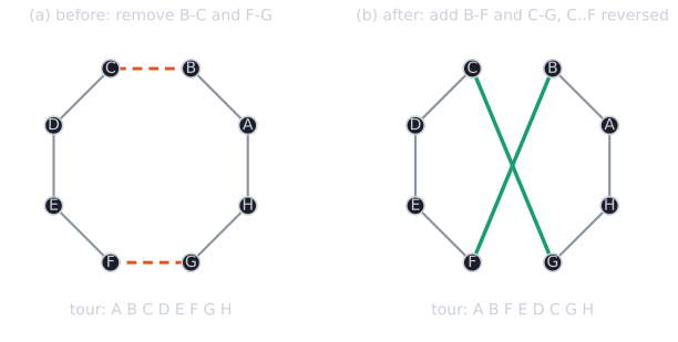
Two facts follow from this picture.
- A move is cheap to evaluate. Only four edges change, so the change in tour length is $$\Delta = d(B, F) + d(C, G) - d(B, C) - d(F, G),$$ four distance lookups, whatever the number of cities. The reversed segment is traversed in the opposite direction, but with symmetric distances its length does not change. This four-term difference is what the article calls one evaluation.
- The neighborhood has $n(n-3)/2$ members. A tour of $n$ cities has $n$ edges, so there are $\binom{n}{2} = n(n-1)/2$ pairs of edges. The $n$ pairs of adjacent edges, which share a city, cannot be reconnected any other way, so they give no move. That leaves $n(n-1)/2 - n = n(n-3)/2$ moves, and different pairs give different tours. For the eight-city example that is 20; for kroA100 it is $100 \times 97 / 2 = 4{,}850$.
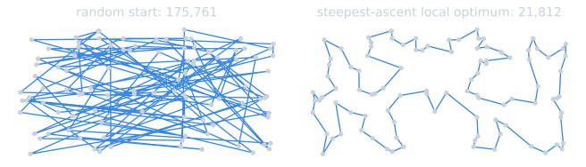
When $\Delta < 0$ the move shortens the tour. A 2-opt local optimum is a tour for which all $n(n-3)/2$ values of $\Delta$ are nonnegative. Geometrically, with Euclidean distances, a tour whose path crosses itself always has an improving 2-opt move. If edges $a\text{-}b$ and $c\text{-}d$ cross at a point $X$, the triangle inequality gives $d(a, c) \le d(a, X) + d(X, c)$ and $d(b, d) \le d(b, X) + d(X, d)$, and the two right-hand sides add up to $d(a, b) + d(c, d)$; the same holds for the other pairing, so whichever reconnection 2-opt makes is shorter (strictly, unless the points are collinear, and up to the rounding that TSPLIB applies to distances). A 2-opt local optimum therefore does not cross itself, which is why the local optimum pictured later in the article looks tidy even though it is 2.5% longer than the best tour.
Because the state is a complete solution, a local search needs almost no memory: one state, and the best value seen. It also produces an answer at any time, which is why local search is used on problems far too large to search systematically (Russell and Norvig, 2020, §4.1). The names follow the direction of improvement. When $f$ is a fitness to maximize, the search climbs; when it is a cost such as tour length, the same algorithm is called descent. This article writes $f$ as a quantity to maximize, and the TSP examples minimize tour length.
Four variants, completely specified
Every hill climber repeats one step: from the current state $x$, choose a neighbor $y$ by some rule, and move to it if $f(y) > f(x)$. They differ in how $y$ is chosen and therefore in how many neighbors must be evaluated per step. Eiben and Smith (2015, §10.2) call this choice the pivot rule: stop at the first improving neighbor (greedy ascent, also called first improvement) or examine them all and take the best (steepest ascent). Russell and Norvig (2020, §4.1.1) add two randomized variants. A complete specification must also say how ties are broken and when the search stops, since an algorithm that leaves these open is not deterministic given a random seed, and its results cannot be reproduced.
First-improvement hill climbing (sometimes called simple hill climbing).
- Fix an order on the moves, for example the 2-opt moves $(i, j)$ sorted by $i$, then by $j$.
- Scan the neighbors of $x$ in that order. Move to the first neighbor $y$ with $f(y) > f(x)$.
- After a move, start the next scan from the beginning of the order. (A common alternative continues from where the last scan stopped. The two can end at different local optima.)
- Stop when a complete scan finds no improving neighbor.
Steepest-ascent hill climbing.
- Evaluate every neighbor of $x$.
- Let $f^* = \max_{y \in N(x)} f(y)$. If $f^* \le f(x)$, stop.
- Otherwise move to a neighbor with value $f^*$. If several share it, choose by a fixed rule, such as the first in the move order, or uniformly at random.
Stochastic hill climbing (Russell and Norvig, 2020, §4.1.1).
- Evaluate every neighbor of $x$ and collect the improving ones, $U = \{ y \in N(x) : f(y) > f(x) \}$.
- If $U$ is empty, stop.
- Otherwise move to a member of $U$ chosen at random: uniformly, or with probability that increases with the size of the improvement.
First-choice hill climbing (Russell and Norvig, 2020, §4.1.1).
- Generate neighbors of $x$ at random, one at a time, and move to the first one that is better than $x$.
- The stopping rule has to be chosen. If neighbors are drawn without replacement, in a fresh random order at each step, the search knows it is at a local optimum when the order is exhausted. If they are drawn with replacement, it must stop after some fixed number of consecutive failures, and it may then stop at a state that still has an improving neighbor.
Russell and Norvig recommend first-choice hill climbing when a state has very many neighbors, since it usually evaluates only a few of them per step. Stochastic hill climbing, in their account, usually climbs more slowly than steepest ascent but sometimes finds better solutions.
All four stop at a local optimum, a state no neighbor improves on (first-choice only when it draws without replacement), and all four certify it the same way: by evaluating the whole neighborhood once and finding nothing better. That final scan is unavoidable for any variant that stops only at a true local optimum.
A worked example: two pivot rules on a small grid
The difference between the pivot rules is easiest to see on a problem small enough to draw. The states are the cells $(x, y)$ of a 25 by 25 grid, $0 \le x, y \le 24$, and each cell has up to four neighbors, the cells directly above, to the right, below, and to the left, scanned in that order. The objective is an integer height made of four hills, labelled $A$ to $D$, with peaks of 655, 893, 1046, and 669, plus a gentle tilt so that the low ground between the hills is not flat. (The heights are $10 \times$ a sum of four Gaussian bumps and the tilt $0.3x + 0.2y$, rounded to integers; the script named at the end of this section lists the parameters.) Every cell other than the four peaks has a strictly higher neighbor, so the only places a hill climber can stop are the peaks, and $C$, at $(11, 6)$, is the global maximum.
Start both rules at $(17, 4)$, on the lower slope between $C$ and $D$. Steepest ascent reads all four neighbors and takes the highest:
| Step | Cell | $f$ | Up | Right | Down | Left | Move |
|---|---|---|---|---|---|---|---|
| 0 | (17, 4) | 471 | 532 | 463 | 389 | 524 | up |
| 1 | (17, 5) | 532 | 556 | 536 | 471 | 582 | left |
| 2 | (16, 5) | 582 | 605 | 532 | 524 | 679 | left |
| 3 | (15, 5) | 679 | 702 | 582 | 617 | 797 | left |
| 4 | (14, 5) | 797 | 824 | 679 | 727 | 909 | left |
| 5 | (13, 5) | 909 | 939 | 797 | 829 | 987 | left |
| 6 | (12, 5) | 987 | 1019 | 909 | 900 | 1013 | up |
| 7 | (12, 6) | 1019 | 992 | 939 | 987 | 1046 | left |
| 8 | (11, 6) | 1046 | 1018 | 1019 | 1013 | 1012 | stop |
It reaches the global maximum $C$ in 8 moves, having evaluated $9 \times 4 = 36$ neighbors, including the final scan at $(11, 6)$ that finds nothing higher. First improvement scans the same neighbors in the same order but takes the first one that is higher than the current cell:
| Step | Cell | $f$ | Neighbors read | First higher neighbor | Move |
|---|---|---|---|---|---|
| 0 | (17, 4) | 471 | up | up 532 | up |
| 1 | (17, 5) | 532 | up | up 556 | up |
| 2 | (17, 6) | 556 | up, right | right 565 | right |
| 3 | (18, 6) | 565 | up, right | right 614 | right |
| 4 | (19, 6) | 614 | up, right | right 662 | right |
| 5 | (20, 6) | 662 | up, right | right 669 | right |
| 6 | (21, 6) | 669 | all four | none | stop |
The two runs part company at step 1. At $(17, 5)$ the cell above is higher (556 against 532), so first improvement takes it, although the cell to the left is higher still (582). That one choice puts it on the slope of $D$, and it climbs to $D$'s peak of 669 in 6 moves and 14 evaluations. Steepest ascent spent 36 evaluations and reached a peak more than half as high again. Neither outcome is a property of the start alone: it is a property of the start together with the pivot rule.
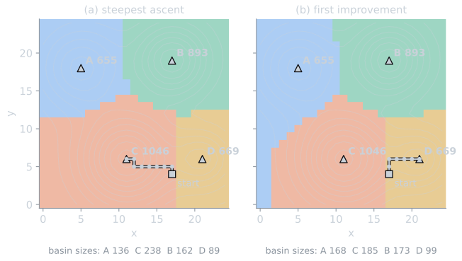
Running both rules from all 625 cells gives their basins of attraction, the sets of starts that end at each peak. Under steepest ascent, 238 of the 625 starts (38.1%) end at $C$; under first improvement, only 185 (29.6%). The basins have different shapes because first improvement always prefers whichever direction is scanned first, here up, so it follows that direction even when another neighbor is much higher. Averaged over all starts, steepest ascent made 6.62 moves and 30.24 evaluations per climb, and first improvement 6.72 moves and 18.88 evaluations. Fewer evaluations per move but a smaller chance of reaching the best peak is the same trade-off that the TSP experiment below measures on a much larger neighborhood. The numbers come from tools/experiments/evolution/hill_climbing_examples.py in the site repository.
Cost per step against number of steps
The cost of a hill climb is the number of steps times the cost of a step, and the variants trade one against the other. Steepest ascent takes the largest improvement available, so it needs few steps, but every step costs a full scan of the neighborhood. First-improvement and first-choice take smaller improvements, so they need more steps, but a step ends as soon as an improvement turns up, which early in a climb is almost immediately.
The four variants were run on kroA100 with the 2-opt neighborhood. Each of 30 seeded runs started all four from the same random tour, and an evaluation is the computation of one move's change in tour length. First-choice drew moves without replacement, steepest ascent broke ties by move order, and stochastic hill climbing chose uniformly among improving moves. Medians, with interquartile ranges in parentheses:
| Variant | Steps | Evaluations | Evaluations per step | Final tour above optimum |
|---|---|---|---|---|
| First-improvement | 390 (376 to 407) | 591,039 (505,596 to 692,742) | 1,589 (1,227 to 1,771) | 5.63% (3.43 to 7.59) |
| Steepest ascent | 104 (102 to 108) | 506,825 (499,550 to 527,438) | 4,897 (4,895 to 4,898) | 6.80% (4.56 to 8.79) |
| First-choice | 330 (312 to 342) | 29,974 (27,841 to 32,519) | 92 (84 to 104) | 10.93% (6.09 to 13.47) |
| Stochastic | 329 (314 to 342) | 1,600,500 (1,525,325 to 1,664,762) | 4,865 (4,864 to 4,865) | 8.50% (5.84 to 12.67) |
Several things are visible. Steepest ascent took a quarter as many steps as first-improvement but used about as many evaluations, because each of its steps cost the full 4,850 (the ratio is slightly above 4,850 because the per-run ratio counts the final scan, which made no move). First-improvement's cost per step is high for a different reason: it restarts its scan from the first move after every step, and near the end of a climb the improving moves are few and late in the order. First-choice, which looks at moves in random order, found an improvement after about 92 evaluations per step, and the whole climb cost about one seventeenth of steepest ascent's. Stochastic hill climbing combined the worst of both: as many steps as first-choice, at the full cost of steepest ascent.
Cheaper climbs did not give equally good tours. The first-choice tours were the longest, a median of 10.9% above the optimum against 5.6% for first-improvement. The interquartile ranges overlap, and this is one instance, so the ordering of tour quality is suggestive rather than settled. What is settled is the cost: per unit of computation, first-choice is far cheaper, which makes it attractive as the inner loop of a method that climbs many times, such as random restarts. The comparison changes with the neighborhood. A larger neighborhood, such as 3-opt, has fewer local optima but costs more per scan, and fast TSP implementations cut the scan cost with candidate lists of each city's nearest neighbors (Lourenço, Martin, and Stützle, 2003). The script is tools/experiments/evolution/hill_climbing.py in the site repository.
One run, step by step
The medians hide the shape of a climb. The figure below follows the four variants through a single run, the first of the 30, all starting from the same random tour of length 175,761, which is more than eight times the optimum. The horizontal axis counts evaluations on a logarithmic scale, so each variant's curve shows how much computation it spent to reach each tour length.
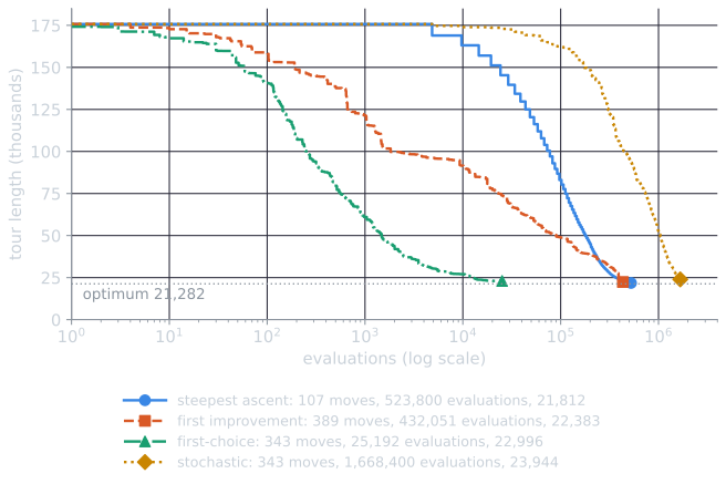
Steepest ascent makes its first move only after evaluating all 4,850 neighbors, so its curve is flat until then; after that, each move removes the worst remaining pair of edges, and the tour shrinks quickly in length per move but slowly per evaluation. First-choice reaches twice the optimum length after 2,010 evaluations, against 144,444 for first improvement, 208,550 for steepest ascent, and 1,139,750 for stochastic hill climbing. In this run steepest ascent ended best, at 21,812 (2.49% above the optimum), first improvement at 22,383, first-choice at 22,996, and stochastic hill climbing at 23,944. Single runs vary a great deal, which is why the table reports medians over 30.
Where hill climbing gets stuck
A hill climber that accepts only strict improvements stops at the first local optimum it reaches. The structure of the fitness landscape decides how often that is a poor place to stop. Russell and Norvig (2020, §4.1.1) name three features. The first two can be seen together on a one-dimensional example, in the spirit of their one-dimensional state-space picture but with numbers that can be checked. The states are the integers $x = 0, 1, \ldots, 60$, the neighbors of $x$ are $x - 1$ and $x + 1$, and $f$ is the piecewise-linear profile drawn below, with integer values from 3 to 21.
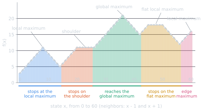
Strict steepest ascent (moving to the higher neighbor while it is strictly higher, and to the left one on a tie) reaches the global maximum from 17 of the 61 starting points, 27.9%. The other 44 starts are lost to four different features, and each needs a different remedy, as the rest of this section and escaping local optima explain.
Local maxima. A local maximum is higher than all its neighbors but lower than the global maximum. Every run in the table above ended at a 2-opt local optimum that was not the global one. On the 8-queens problem, Russell and Norvig's running example, the objective is the number of pairs of queens that attack each other, to be minimized. Steepest descent from a random placement reaches a solution only about 14% of the time and stops at a local minimum otherwise, after a climb of only three or four moves (hill climbing on 8-queens and the 8-puzzle reproduces this over 30,000 runs).
Plateaus. A plateau is a region of neighboring states with equal value. Two kinds are worth distinguishing. A flat local maximum has no higher neighbor anywhere on its edge, so no amount of wandering helps. A shoulder is a plateau with an uphill edge somewhere, so progress is possible if the search keeps moving. A strict hill climber stops on both. Allowing sideways moves to neighbors of equal value lets it cross a shoulder, but on a flat maximum it would wander forever, so the number of consecutive sideways moves must be capped. The 8-queens problem has many shoulders, and allowing up to 100 consecutive sideways moves raises the success rate of steepest descent from about 14% to about 94%, at the price of longer climbs (escaping local optima gives the numbers).
The one-dimensional example shows both kinds and makes the cap concrete. Its shoulder runs from $x = 20$ to $x = 26$ at height 11, and $x = 27$ is higher. A climber that arrives at $x = 20$ from the left has one neighbor of equal value, $x = 21$; inside the shoulder it has two, and with random tie-breaking it steps left or right with probability $\tfrac{1}{2}$ each; at $x = 26$ the uphill exit appears. The sideways moves therefore form a symmetric random walk on the seven states 20 to 26, turned back at 20 and ending at 26. The expected number of steps for such a walk to cover a distance $m$ is $m^2$, here $6^2 = 36$ sideways moves, and propagating the walk's distribution exactly gives a probability of 0.9612 of reaching $x = 26$ within a cap of 100. On the flat maximum from 45 to 50, by contrast, both edges lead down, and the same walk spends the whole budget of 100 moves going back and forth before it stops. With the cap at 100, the probability of reaching the global maximum from a uniformly random start rises from 0.2787 to 0.4527 (the walk was computed with random tie-breaking throughout, so the two valley points $x = 14$ and $x = 42$ now go either way with equal probability). The starts from 0 to 13, which climb to $x = 8$, and the 18 starts from 43 to 60, which end on the flat maximum or the edge maximum, are not helped at all: their climbs end where every way out goes down.
Ridges. A ridge is a sequence of local maxima that rises, but in a direction no single move follows. A small example makes the geometry concrete. On the integer grid $0 \le x, y \le 10$, let
$$f(x, y) = (x + y) - 10\,(x - y)^2,$$
with moves that change one coordinate by $\pm 1$. Along the diagonal, $f(k, k) = 2k$, rising from 0 to 20. But from any diagonal point, every move leaves the diagonal: $f(k + 1, k) = 2k + 1 - 10 = 2k - 9$, which is lower. Every diagonal point is therefore a local maximum, and a hill climber started at $(0, 0)$ stops at once with $f = 0$, although $f(10, 10) = 20$. A move along the diagonal, changing both coordinates at once, would climb the ridge directly. The ridge is a property of the objective together with the move set, as all of these features are.
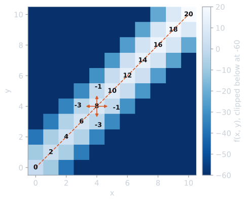
In two dimensions the remedy looks obvious: add the diagonal move. In a problem with thousands of variables, the useful combined moves are not known in advance, and adding all combinations makes the neighborhood too large to scan. This is the general tension in choosing a neighborhood: a small one is cheap to scan and has many local optima, a large one has fewer local optima and is expensive.
The (1+1) EA: a hill climber with a global mutation operator
The simplest evolutionary algorithm differs from a stochastic hill climber in one respect. The $(1+1)$ EA on bitstrings of length $n$ keeps one parent $x$, creates one child $y$ by flipping each bit independently with probability $1/n$, and replaces $x$ by $y$ if $f(y) \ge f(x)$ (Droste, Jansen, and Wegener, 2002). It is the bitstring counterpart of the $(1+1)$ evolution strategy from the early history of evolutionary computation. Compare it with randomized local search, which flips exactly one bit chosen uniformly at random and makes the same acceptance test. Apart from accepting moves to equal values, which lets it drift across plateaus, randomized local search is first-choice hill climbing with sampling with replacement and no stopping rule.
The difference lies in the neighborhood. Randomized local search can reach only the $n$ strings at Hamming distance 1. The mutation operator of the $(1+1)$ EA can produce any string at all: a particular string at Hamming distance $k$ arises with probability
$$\left(\frac{1}{n}\right)^{k} \left(1 - \frac{1}{n}\right)^{n-k},$$
which is never zero: the $k$ chosen bits must all flip, each with probability $1/n$, and the other $n - k$ must all stay, each with probability $1 - 1/n$. For $n = 100$ the probability is about 0.0037 for one particular string one bit away, $3.7 \times 10^{-5}$ for one two bits away, and $3.8 \times 10^{-7}$ for one three bits away, so the expected numbers of tries to hit that string are about 270, 26,800, and 2,651,000 (values rounded; the script tools/experiments/evolution/hill_climbing_examples.py computes them). About 37% of children, a fraction $(1 - 1/n)^n \approx 1/e$, are exact copies of the parent. The operator is called global because no string has probability zero. Under it, every state is a neighbor of every other, so in the strict sense of the definition the $(1+1)$ EA has no local optima except the global ones. What it has instead is waiting times. If the only improvement on a state lies $k$ bits away, the probability of producing it in one step is at most $n^{-k}$, so the expected wait is at least $n^k$ steps. Droste, Jansen, and Wegener (2002) made this exact with the functions $\mathrm{Jump}_m$, which rise with the number of ones except for a gap of width $m$ just below the all-ones optimum. They proved that the expected optimization time of the $(1+1)$ EA on $\mathrm{Jump}_m$ is $\Theta(n^m + n \log n)$. For $m = 1$ that is the $\Theta(n \log n)$ of OneMax, and for the trap function, where the gap spans the whole space, it is $\Theta(n^n)$. Randomized local search, by contrast, once it reaches the edge of a gap of width 2 or more, never crosses it.
So the $(1+1)$ EA is best read as a stochastic hill climber on a weighted neighborhood: it mostly makes one- or two-bit moves, and occasionally a long jump. Fitness landscapes shows the consequence on NK problems, where most of the runs that found the global optimum had passed through a local optimum of the one-bit-flip neighborhood on the way. The $(1+1)$ EA also shows why the fitness landscape depends on the algorithm: the same function can have thousands of local optima for randomized local search and none, strictly speaking, for the $(1+1)$ EA.
Hill climbing elsewhere
Hill climbing appears inside many algorithms that are not usually called by that name. K-means is one. Lloyd's algorithm alternates two steps, neither of which can raise the residual sum of squares, and it stops when neither step changes anything. That point is a local minimum of the objective with respect to those two steps, not necessarily the global minimum, and the standard remedy, running K-means from several starting points and keeping the best result, is random-restart hill climbing (K-means in practice measures how much the start matters on Reuters). Some evolutionary algorithms also apply a hill climber to each offspring before it competes. Eiben and Smith (2015, ch. 10) treat these hybrids as memetic algorithms, in which local search refines what the evolutionary search finds.
The common lesson is the one this topic is built around. Hill climbing is fast, and on smooth problems it is enough. Its weakness is that it cannot accept a worse state, so it ends wherever the first local optimum lies. Escaping local optima covers the main remedies: sideways moves, restarts, simulated annealing, tabu search, iterated local search, and finally the population of an evolutionary algorithm. Hill climbing on 8-queens and the 8-puzzle applies steepest descent to two classic puzzles.
References
- Croes, G. A. (1958). A method for solving traveling-salesman problems. Operations Research, 6(6), 791–812.
- Droste, S., Jansen, T., and Wegener, I. (2002). On the analysis of the (1+1) evolutionary algorithm. Theoretical Computer Science, 276(1–2), 51–81.
- Eiben, A. E., and Smith, J. E. (2015). Introduction to Evolutionary Computing, 2nd ed., chapter 10. Springer.
- Lin, S. (1965). Computer solutions of the traveling salesman problem. Bell System Technical Journal, 44(10), 2245–2269.
- Lourenço, H. R., Martin, O. C., and Stützle, T. (2003). Iterated local search. In F. Glover and G. A. Kochenberger (Eds.), Handbook of Metaheuristics, 320–353. Kluwer Academic Publishers.
- Reinelt, G. (1991). TSPLIB: A traveling salesman problem library. ORSA Journal on Computing, 3(4), 376–384.
- Russell, S., and Norvig, P. (2020). Artificial Intelligence: A Modern Approach, 4th ed., section 4.1. Pearson.