K-means produces a flat set of $K$ clusters. Many uses of clustering want a hierarchy instead: broad groups at the top for an overview, divided into narrower ones for a closer look. Browsing a collection works this way, and so do taxonomies of topics; the original Scatter/Gather system produced such levels on the fly, by reclustering the groups a user selected. Hierarchical clustering builds that structure directly, as a tree of nested clusters, and does not need the number of clusters in advance. This article follows Manning, Raghavan, and Schütze (2008, chapter 17), and traces every method by hand on six points before comparing them on news stories.
Agglomerative clustering
The common approach is bottom-up, or hierarchical agglomerative clustering (HAC):
- Start with every document in a cluster of its own.
- Find the two most similar clusters and merge them.
- Repeat until a single cluster contains everything.
Each merge is recorded, so the result is a binary tree with documents at the leaves and the whole collection at the root. $N$ documents take exactly $N - 1$ merges. Unlike K-means, HAC has no random starting point. Given the same documents and similarity measure, it always produces the same tree, apart from ties.
The opposite, top-down approach is divisive clustering: start with one cluster and repeatedly split one in two, for example with K-means using $K = 2$ (bisecting K-means). It is less common, though Steinbach, Karypis, and Kumar (2000) found bisecting K-means competitive with the best agglomerative methods on text, and it can be faster when only the top levels of the tree are needed.
Similarity between clusters
Step 2 needs the similarity of two clusters, not only of two documents. The choice, called the linkage, decides what the algorithm finds. With document similarity measured by cosine similarity:
- Single linkage uses the similarity of the most similar pair, one document from each cluster. Two clusters are close if any of their members are close.
- Complete linkage uses the similarity of the least similar pair. Two clusters are close only if all their members are close.
- Average linkage uses the average similarity over all pairs with one document in each cluster. The textbook's group-average variant averages over all pairs in the merged cluster, including pairs within each original cluster.
- Centroid linkage uses the similarity of the two clusters' centroids. With dot-product similarity on unit vectors, the average over cross pairs equals the dot product of the two centroids (Manning, Raghavan, and Schütze, 2008, §17.4), so average linkage in this form and centroid linkage coincide. When centroids are compared by a distance instead, centroid linkage behaves differently, as the section on inversions below shows.
Everything here can be stated with distances instead of similarities, merging the two closest clusters: single linkage then uses the smallest cross-pair distance, complete linkage the largest, and so on. The worked example uses distances, because points on a line make them easy to read.
A worked example
Six points on a line, at $a = 0$, $b = 1$, $c = 2.5$, $d = 4.5$, $e = 5.7$ and $f = 9.5$, with the distance between two points the difference of their positions. They form a loose chain from $a$ to $e$, with $f$ off on its own:
| a | b | c | d | e | f | |
|---|---|---|---|---|---|---|
| a | 0 | 1 | 2.5 | 4.5 | 5.7 | 9.5 |
| b | 1 | 0 | 1.5 | 3.5 | 4.7 | 8.5 |
| c | 2.5 | 1.5 | 0 | 2 | 3.2 | 7 |
| d | 4.5 | 3.5 | 2 | 0 | 1.2 | 5 |
| e | 5.7 | 4.7 | 3.2 | 1.2 | 0 | 3.8 |
| f | 9.5 | 8.5 | 7 | 5 | 3.8 | 0 |
The first two merges are the same for every linkage, because between single points all linkages agree: the smallest entry is $a$–$b$ at 1, then $d$–$e$ at 1.2.
The third merge joins $c$ to $\{a, b\}$ under every linkage, but at different heights, because the linkages measure the distance from $c$ to $\{a, b\}$ differently. The two cross distances are $c$–$b$ = 1.5 and $c$–$a$ = 2.5. Single linkage takes the smaller, 1.5; complete the larger, 2.5; average their mean, 2.0. In each case this is the smallest distance among the clusters left, $\{a, b\}$, $c$, $\{d, e\}$, $f$.
The fourth merge is where the linkages disagree. Three clusters remain besides the trivial ones, $\{a, b, c\}$, $\{d, e\}$ and $f$, and the candidate distances are:
| Pair | Cross distances | Single | Complete | Average |
|---|---|---|---|---|
| {a, b, c} and {d, e} | 4.5, 5.7, 3.5, 4.7, 2, 3.2 | 2 | 5.7 | 3.93 |
| {d, e} and f | 5, 3.8 | 3.8 | 5 | 4.4 |
| {a, b, c} and f | 9.5, 8.5, 7 | 7 | 9.5 | 8.33 |
Single linkage sees the close pair $c$–$d$ at distance 2 and joins the chain. Complete linkage sees that $a$ and $e$ are 5.7 apart, which would make $\{a, \dots, e\}$ a wide cluster, and prefers $\{d, e, f\}$, whose widest pair is 5. Average linkage, at $23.6 / 6 \approx 3.93$ against 4.4, sides with single linkage this time. The full sequence of merges, with the distance at which each happened (rounded to two decimals):
| Merge | Single link | Complete link | Average link |
|---|---|---|---|
| 1 | a + b at 1 | a + b at 1 | a + b at 1 |
| 2 | d + e at 1.2 | d + e at 1.2 | d + e at 1.2 |
| 3 | ab + c at 1.5 | ab + c at 2.5 | ab + c at 2 |
| 4 | abc + de at 2 | de + f at 5 | abc + de at 3.93 |
| 5 | abcde + f at 3.8 | abc + def at 9.5 | abcde + f at 6.76 |
Centroid linkage gives the same tree as average linkage here. On a line, the distance between two centroids equals the average cross distance whenever one cluster lies entirely to one side of the other, which is true at every merge of this example. In the plane the two differ.
Dendrograms
The tree is drawn as a dendrogram, with documents along the bottom and each merge drawn as a horizontal line joining two branches, at a height given by the distance (or similarity) of the clusters merged. Merges of very similar clusters sit near the bottom; the last, least similar merges sit near the top.
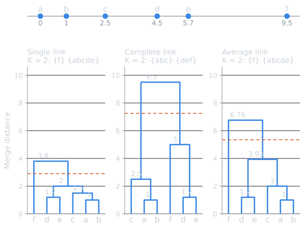
A flat clustering can be taken from the tree by cutting it:
- at a fixed similarity, keeping only merges above a threshold;
- at the number of clusters wanted, undoing the last $K - 1$ merges;
- at the largest gap between successive merge heights, where the next merge would join clusters much less similar than any merged before.
In the example, all three trees have their largest gap before the last merge (from 2 to 3.8 for single link, 5 to 9.5 for complete, 3.93 to 6.76 for average), so the gap rule gives two clusters in each case: $\{a, b, c, d, e\}$ and $\{f\}$ for single and average linkage, $\{a, b, c\}$ and $\{d, e, f\}$ for complete. The tree holds every one of these clusterings at once, which is part of its appeal. A browsing interface can show the top levels and let users descend.
Updating cluster distances
After a merge, HAC needs the distance from the new cluster $i \cup j$ to every other cluster $k$. Recomputing it from all document pairs would be slow, but each linkage has a rule that uses only the distances already known (sizes are written $n_i$, $n_j$):
| Linkage | Distance from $k$ to the merged cluster $i \cup j$ |
|---|---|
| Single | $\min(D_{ki}, D_{kj})$ |
| Complete | $\max(D_{ki}, D_{kj})$ |
| Average | $\dfrac{n_i D_{ki} + n_j D_{kj}}{n_i + n_j}$ |
The average rule holds because the cross pairs between $k$ and $i \cup j$ are the cross pairs with $i$ plus those with $j$, so their mean is the size-weighted mean of the two averages. In the example, after $\{a, b, c\}$ and $\{d, e\}$ merge, the distance from $f$ to the new cluster is $(3 \times 8.33 + 2 \times 4.4) / 5 = 6.76$, matching the last merge in the table.
For group-average clustering with dot-product similarity, the textbook gives an even cheaper form: the sum of the dot products of all pairs of distinct documents in a cluster, counting each pair in both orders, equals the squared length of the cluster's vector sum minus the self-similarities, so keeping one vector sum per cluster gives each cluster similarity in constant time (Manning, Raghavan, and Schütze, 2008, §17.3).
Centroid linkage and inversions
The rule for centroid linkage, with squared Euclidean distances between centroids, is the one place where something surprising happens. Write $\vec{\mu}_i$, $\vec{\mu}_j$, $\vec{\mu}_k$ for the centroids and $n = n_i + n_j$. The merged centroid is $\vec{m} = (n_i \vec{\mu}_i + n_j \vec{\mu}_j)/n$, so
$$\vec{\mu}_k - \vec{m} = \frac{n_i}{n} (\vec{\mu}_k - \vec{\mu}_i) + \frac{n_j}{n} (\vec{\mu}_k - \vec{\mu}_j).$$
Squaring, and writing the cross term with $\vec{u} = \vec{\mu}_k - \vec{\mu}_i$ and $\vec{w} = \vec{\mu}_k - \vec{\mu}_j$ as $2\,\vec{u} \cdot \vec{w} = \lvert \vec{u} \rvert^2 + \lvert \vec{w} \rvert^2 - \lvert \vec{u} - \vec{w} \rvert^2$, where $\vec{u} - \vec{w} = \vec{\mu}_j - \vec{\mu}_i$, gives
$$\lvert \vec{\mu}_k - \vec{m} \rvert^2 = \frac{n_i}{n} \lvert \vec{\mu}_k - \vec{\mu}_i \rvert^2 + \frac{n_j}{n} \lvert \vec{\mu}_k - \vec{\mu}_j \rvert^2 - \frac{n_i n_j}{n^2} \lvert \vec{\mu}_i - \vec{\mu}_j \rvert^2.$$
The first two terms are a weighted average, like the average-linkage rule. The third is subtracted, and it is large when the two clusters just merged were far apart. That can make the new cluster closer to $k$ than $i$ and $j$ were to each other.
Three points show it. Put $d_1 = (0, 0)$, $d_2 = (4, 0)$ and $d_3 = (2, 3.6)$. The closest pair is $d_1$, $d_2$ at distance 4 ($d_3$ is $\sqrt{2^2 + 3.6^2} \approx 4.12$ from each). Their centroid is $(2, 0)$, which is only 3.6 from $d_3$. By the formula, $\tfrac{1}{2}(16.96) + \tfrac{1}{2}(16.96) - \tfrac{1}{4}(16) = 12.96 = 3.6^2$. So the second merge happens at a smaller distance, 3.6, than the first, 4. This is an inversion: in the dendrogram the second merge line is drawn below the first, and the tree no longer says that clusters merged later are less alike (Manning, Raghavan, and Schütze, 2008, §17.4, give an example of the same shape).
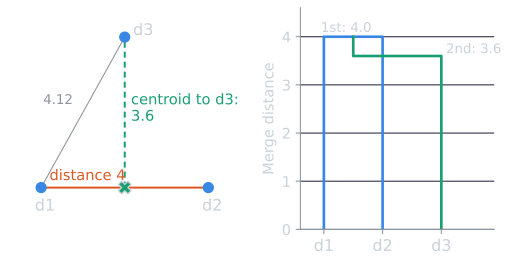
Single, complete and average linkage cannot invert. Suppose $i$ and $j$ were merged because $D_{ij}$ was the smallest distance between any two clusters, so $D_{ki} \ge D_{ij}$ and $D_{kj} \ge D_{ij}$ for every other $k$. The minimum, maximum, and any weighted average of two numbers that are both at least $D_{ij}$ are also at least $D_{ij}$. Every distance after the merge is therefore at least as large as the distance just merged at, and merge heights can only rise. With dot-product similarity, centroid linkage cannot invert either, because the similarity of a centroid to a merged centroid is the size-weighted average of its similarities to the two parts, with no subtracted term.
Chaining and outliers
Single linkage has a well-known weakness, chaining. Because one close pair is enough to merge two clusters, a sequence of documents each similar to the next can join documents at the two ends that have nothing in common. The example shows it at small scale: single linkage puts $a$ and $e$ in one cluster although they are 5.7 apart, farther than $e$ is from $f$, because each link along the chain is at most 2. Single-link clusters tend to be long and straggly, and on text it often grows one giant cluster that absorbs documents one at a time. Single-link HAC is equivalent to building a minimum spanning tree of the documents and removing its longest edges.
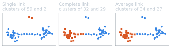
Complete linkage avoids chaining. It prefers compact clusters with small diameters, but it is sensitive to outliers. A single document far from the rest greatly increases the diameter of any cluster it could join, and can change the whole clustering, as $f$ does in the example by pulling $d$ and $e$ away from $c$. Average linkage is a compromise between the two, and Manning, Raghavan, and Schütze (2008, chapter 17) recommend group-average clustering for documents.
Cost
Naive HAC computes all $N^2$ document similarities, then at each of $N - 1$ merges scans every pair of clusters for the most similar. With $m$ clusters left, a scan looks at about $m^2/2$ pairs, and adding this up for $m = N, N - 1, \dots, 2$ gives about $N^3/6$ comparisons, $O(N^3)$ in total.
The priority-queue algorithm avoids the repeated scans (Manning, Raghavan, and Schütze, 2008, §17.2.1). Each cluster keeps its similarities to all other clusters in a priority queue, so its best partner is always at the front.
- Build one queue per document, holding its similarities to the other $N - 1$ documents: $O(N^2 \log N)$ in all, or $O(N^2)$ with a heap built in linear time.
- To find the next merge, look at the front of each of the at most $N$ queues and take the best: $O(N)$.
- After merging $i$ and $j$, go through every other cluster $k$: delete its entries for $i$ and $j$, compute the distance to the new cluster with the update rule above, and insert it. That is a constant number of queue operations, $O(\log N)$ each, for each of up to $N$ clusters: $O(N \log N)$ per merge. The new cluster gets a fresh queue built from the same values.
With $N - 1$ merges, the total is $O(N^2 \log N)$. In the example, $c$'s queue starts as $b$ 1.5, $d$ 2, $a$ 2.5, $e$ 3.2, $f$ 7, nearest first. When $a$ and $b$ merge, the entries for $a$ and $b$ are deleted and one for $\{a, b\}$ is inserted: at 1.5 under single linkage, which goes to the front, and at 2.5 under complete linkage, which goes behind $d$.
Single linkage can be done in $O(N^2)$. It has a property the others lack, which the textbook calls best-merge persistence: if $j$ is the best partner of $k$, and $j$ then merges with some other cluster, the merged cluster is still the best partner of $k$, since single-link distance to it is the smaller of the two old distances. It is therefore enough to remember one best partner per cluster instead of a whole queue (Manning, Raghavan, and Schütze, 2008, §17.2.1). Complete linkage does not have this property, because a merge can make a cluster's former best partner worse. In practice the difference matters less than the notation suggests: all these algorithms compute $O(N^2)$ document similarities, and computing a similarity between two documents costs far more than a comparison inside a queue. They also keep the $N \times N$ similarity matrix, so memory is quadratic as well.
That cost decides when HAC can be used. For the few hundred results of a query, it is fast: 600 documents have about 180,000 distinct pairs. For a collection of a million documents, the similarity matrix has $5 \times 10^{11}$ distinct pairs, about 2 terabytes at four bytes each, and K-means, linear in $N$, is the practical choice. A common hybrid clusters a sample with HAC, uses the resulting clusters as starting centroids, and runs K-means on the whole collection. The Buckshot algorithm of Scatter/Gather works this way (Cutting, Karger, Pedersen, and Tukey, 1992).
Comparison on Reuters
The four methods were compared on a random sample of 600 stories from the six-category Reuters collection of K-means in practice, with the same TF-IDF vectors, about half of them in the large earn category. Each dendrogram was cut into six clusters, and the lowest-RSS of ten k-means++ runs on the same sample was taken for comparison. The measures are defined in evaluating clusterings.
| Method | Purity | NMI | Rand index | Cluster sizes |
|---|---|---|---|---|
| Single linkage | 0.523 | 0.018 | 0.379 | 595, 1, 1, 1, 1, 1 |
| Complete linkage | 0.532 | 0.036 | 0.394 | 577, 9, 5, 4, 3, 2 |
| Average (centroid) linkage | 0.725 | 0.369 | 0.689 | 308, 261, 9, 9, 8, 5 |
| K-means | 0.753 | 0.409 | 0.691 |
Single linkage chained almost everything into one cluster and left five individual stories apart at the top of the tree, the same behaviour as in the chaining figure, at scale. Its NMI of 0.018 says the clusters carry almost no information about the categories. Complete linkage ran into a property of sparse text vectors. Many pairs of stories share no terms and have similarity exactly zero, and once clusters grow, nearly every pair of clusters contains such a pair. The last 27 merges all took place at complete-link similarity zero, so which clusters merged, and the six-cluster cut, were decided by how ties were broken, not by the data. In both cases the cut at six clusters does not reflect the categories, though the trees may hold sensible groups at lower levels.
Average linkage produced two large clusters and four small ones, with scores close to K-means. K-means was slightly better on all three measures. On this collection the choice of linkage mattered far more than the choice between average-link HAC and K-means.
When to use which
- Hierarchical clustering suits small collections, such as a set of search results, and uses that need a hierarchy or an unknown number of clusters. It is deterministic, which makes results reproducible.
- K-means suits large collections and uses that need a fixed number of flat clusters. It is fast but depends on its starting point.
- Average linkage is the safest default for text. Single linkage is useful mainly for its connection to minimum spanning trees and for finding elongated structures, not for grouping documents by topic.
The worked example and the inversion are recomputed by tools/experiments/clustering/hac_toy.py, and the Reuters comparison by tools/experiments/clustering/reuters_kmeans.py, in the site repository.
References
- Cutting, D. R., Karger, D. R., Pedersen, J. O., and Tukey, J. W. (1992). Scatter/Gather: A cluster-based approach to browsing large document collections. In Proceedings of SIGIR 1992, 318–329.
- Manning, C. D., Raghavan, P., and Schütze, H. (2008). Introduction to Information Retrieval, chapter 17. Cambridge University Press.
- Steinbach, M., Karypis, G., and Kumar, V. (2000). A comparison of document clustering techniques. In KDD Workshop on Text Mining.